I-1 The optimal Mercator projection (UM) 629
J lA :
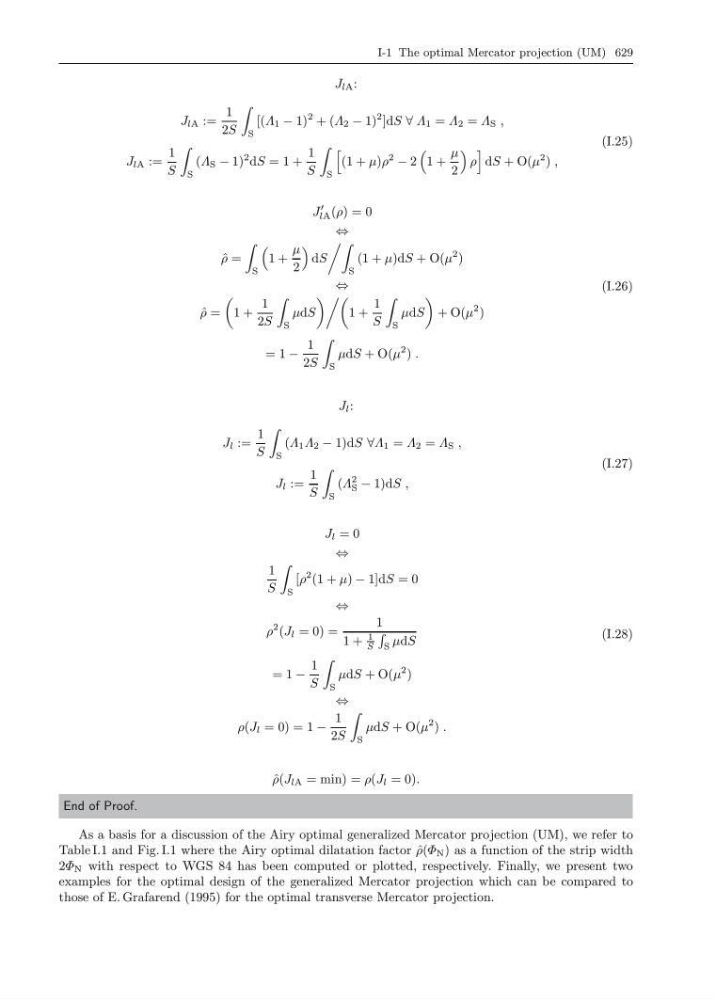
J lA :=
1
2S
S
[(Λ 1 − 1)
2 + (Λ 2 − 1)
2 ]dS ∀ Λ 1 = Λ 2 = Λ S ,
J lA :=
1
S
S
(Λ S − 1)
2 dS = 1 +
1
S
S
(1 + µ)ρ
2
− 2
1 +
µ
2
ρ
dS + O(µ
2 ) ,
(I.25)
J
lA (ρ) = 0
⇔
ˆ
ρ =
S
1 +
µ
2
dS
S
(1 + µ)dS + O(µ
2 )
⇔
ˆ
ρ =
1 +
1
2S
S
µdS
1 +
1
S
S
µdS
+ O(µ
2 )
= 1 −
1
2S
S
µdS + O(µ
2 ) .
(I.26)
J l :
J l :=
1
S
S
(Λ 1 Λ 2 − 1)dS ∀Λ 1 = Λ 2 = Λ S ,
J l :=
1
S
S
(Λ
2
S − 1)dS ,
(I.27)
J l = 0
⇔
1
S
S
[ρ
2 (1 + µ) − 1]dS = 0
⇔
ρ
2 (J l = 0) =
1
1 +
1
S
S
µdS
= 1 −
1
S
S
µdS + O(µ
2 )
⇔
ρ(J l = 0) = 1 −
1
2S
S
µdS + O(µ
2 ) .
(I.28)
ˆ
ρ(J lA = min) = ρ(J l = 0).
End of Proof.
As a basis for a discussion of the Airy optimal generalized Mercator projection (UM), we refer to
Table I.1 and Fig. I.1 where the Airy optimal dilatation factor ˆ
ρ(Φ N ) as a function of the strip width
2Φ N with respect to WGS 84 has been computed or plotted, respectively. Finally, we present two
examples for the optimal design of the generalized Mercator projection which can be compared to
those of E. Grafarend (1995) for the optimal transverse Mercator projection.