596 G Generalized Mollweide projection
As soon as we implement the axe a and the axe b in the generalized Kepler equation (G.31), we gain its
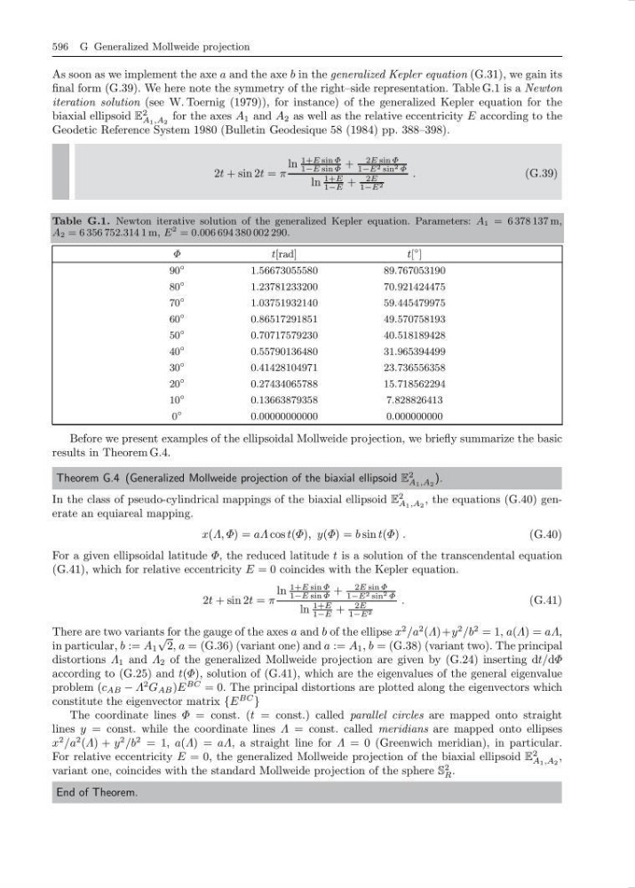
final form (G.39). We here note the symmetry of the right–side representation. Table G.1 is a Newton
iteration solution (see W. Toernig (1979)), for instance) of the generalized Kepler equation for the
biaxial ellipsoid E
2
A 1 ,A 2
for the axes A 1 and A 2 as well as the relative eccentricity E according to the
Geodetic Reference System 1980 (Bulletin Geodesique 58 (1984) pp. 388–398).
2t + sin 2t = π
ln
1+E sin Φ
1−E sin Φ +
2E sin Φ
1−E 2 sin 2 Φ
ln
1+E
1−E +
2E
1−E 2
.
(G.39)
Table G.1. Newton iterative solution of the generalized Kepler equation. Parameters: A 1 = 6 378 137 m,
A 2 = 6 356 752.314 1 m, E
2 = 0.006 694 380 002 290.
Φ
t [rad]
t[
◦ ]
90
◦
1.56673055580
89.767053190
80
◦
1.23781233200
70.921424475
70
◦
1.03751932140
59.445479975
60
◦
0.86517291851
49.570758193
50
◦
0.70717579230
40.518189428
40
◦
0.55790136480
31.965394499
30
◦
0.41428104971
23.736556358
20
◦
0.27434065788
15.718562294
10
◦
0.13663879358
7.828826413
0
◦
0.00000000000
0.000000000
Before we present examples of the ellipsoidal Mollweide projection, we briefly summarize the basic
results in Theorem G.4.
Theorem G.4 (Generalized Mollweide projection of the biaxial ellipsoid E
2
A 1 ,A 2
).
In the class of pseudo-cylindrical mappings of the biaxial ellipsoid E
2
A 1 ,A 2
, the equations (G.40) generate an equiareal mapping.
x(Λ, Φ) = aΛ cos t(Φ), y(Φ) = b sin t(Φ) .
(G.40)
For a given ellipsoidal latitude Φ, the reduced latitude t is a solution of the transcendental equation
(G.41), which for relative eccentricity E = 0 coincides with the Kepler equation.
2t + sin 2t = π
ln
1+E sin Φ
1−E sin Φ +
2E sin Φ
1−E 2 sin 2 Φ
ln
1+E
1−E +
2E
1−E 2
.
(G.41)
There are two variants for the gauge of the axes a and b of the ellipse x
2 /a
2 (Λ)+y
2 /b
2 = 1, a(Λ) = aΛ,
in particular, b := A 1
√
2, a = (G.36) (variant one) and a := A 1 , b = (G.38) (variant two). The principal
distortions Λ 1 and Λ 2 of the generalized Mollweide projection are given by (G.24) inserting dt/dΦ
according to (G.25) and t(Φ), solution of (G.41), which are the eigenvalues of the general eigenvalue
problem (c AB − Λ
2 G AB )E
BC = 0. The principal distortions are plotted along the eigenvectors which
constitute the eigenvector matrix {E
BC
}
The coordinate lines Φ = const. (t = const.) called parallel circles are mapped onto straight
lines y = const. while the coordinate lines Λ = const. called meridians are mapped onto ellipses
x
2 /a
2 (Λ) + y
2 /b
2 = 1, a(Λ) = aΛ, a straight line for Λ = 0 (Greenwich meridian), in particular.
For relative eccentricity E = 0, the generalized Mollweide projection of the biaxial ellipsoid E
2
A 1 ,A 2
,
variant one, coincides with the standard Mollweide projection of the sphere S
2
R .
End of Theorem.