584 F Mixed cylindric map projections
Corollary F.11 (The right eigenvectors of the right Cauchy–Green deformation tensor).
The right eigenvectors of the right Cauchy–Green deformation tensor normalized with respect to the
right metric tensor G r = I 2 can be represented by
f r1 =
−C 12 e 2 + (C 22 − λ
2
1 )e 1
C 2
12 + (C 22 − λ 2
1 ) 2
, f r2 =
−C 12 e 1 + (C 11 − λ
2
2 )e 2
C 2
12 + (C 11 − λ 2
2 ) 2
,
(F.74)
namely with respect to the orthonormal basis {e 1 , e 2 } which spans {R
2 , δ αβ }. The coordinates of the
eigenvectors {f r1 , f r2 } generate the orthonormal matrix
F r =
cos ϕ sin ϕ
− sin ϕ cos ϕ
= [f r1 , f r2 ] ,
(F.75)
such that
tan ϕ =
C 12
−(C 11 − λ 2
2 )
=
2C 12
C 22 − C 11 −
(C 11 − C 22 ) 2 + (2C 12 ) 2
, cot ϕ =
2C 12
C 11 − C 22
. (F.76)
End of Corollary.
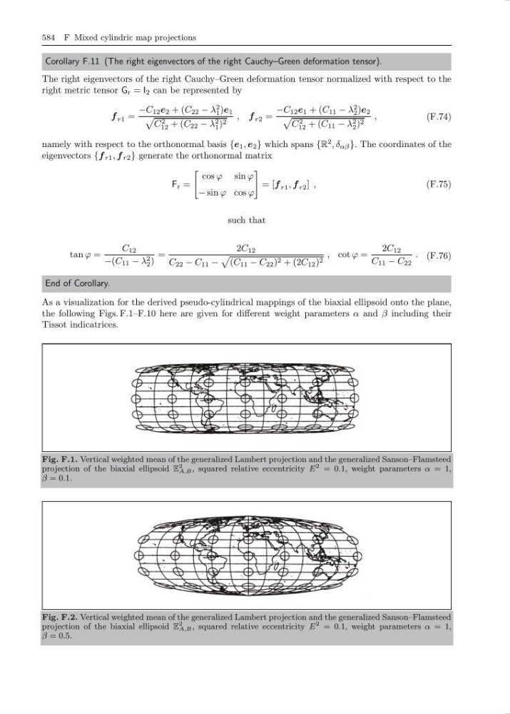
As a visualization for the derived pseudo-cylindrical mappings of the biaxial ellipsoid onto the plane,
the following Figs. F.1–F.10 here are given for different weight parameters α and β including their
Tissot indicatrices.
Fig. F.1. Vertical weighted mean of the generalized Lambert projection and the generalized Sanson–Flamsteed
projection of the biaxial ellipsoid E
2
A,B , squared relative eccentricity E
2 = 0.1, weight parameters α = 1,
β = 0.1.
Fig. F.2. Vertical weighted mean of the generalized Lambert projection and the generalized Sanson–Flamsteed
projection of the biaxial ellipsoid E
2
A,B , squared relative eccentricity E
2 = 0.1, weight parameters α = 1,
β = 0.5.