

E-3 The Newton form of a geodesic in Maupertuis gauge (sphere, ellipsoid-of-revolution) 557
E-34 A geodesic as a submanifold of the ellispoid-of-revolution (conformal coordinates)
Let us represent the differential equations of a geodesic as a submanifold of the ellispoid-of-revolution
M
2 := E
2
A,B as functions q
µ (t) as well as the Lagrangean L
2 and the Hamiltonian H
2 with respect
to conformal coordinates (isothermal, isometric) of the most important applicable map projections
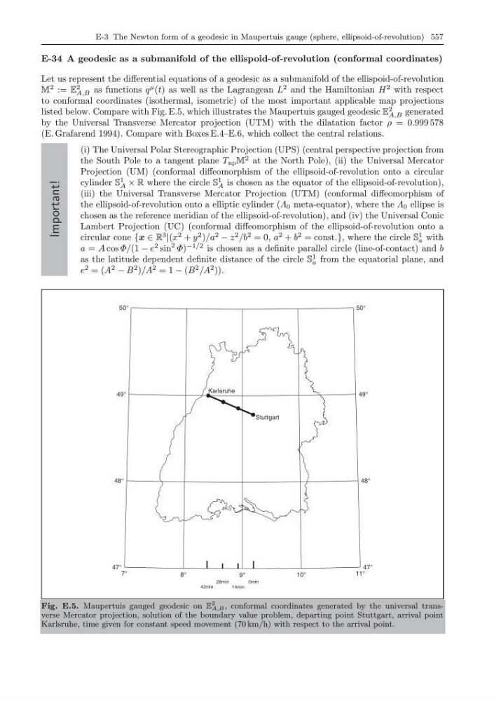
listed below. Compare with Fig. E.5, which illustrates the Maupertuis gauged geodesic E
2
A,B generated
by the Universal Transverse Mercator projection (UTM) with the dilatation factor ρ = 0.999 578
(E. Grafarend 1994). Compare with Boxes E.4–E.6, which collect the central relations.
Important!
(i) The Universal Polar Stereographic Projection (UPS) (central perspective projection from
the South Pole to a tangent plane T np M
2 at the North Pole), (ii) the Universal Mercator
Projection (UM) (conformal diffeomorphism of the ellipsoid-of-revolution onto a circular
cylinder S
1
A × R where the circle S
1
A is chosen as the equator of the ellipsoid-of-revolution),
(iii) the Universal Transverse Mercator Projection (UTM) (conformal diffeomorphism of
the ellipsoid-of-revolution onto a elliptic cylinder (Λ 0 meta-equator), where the Λ 0 ellipse is
chosen as the reference meridian of the ellipsoid-of-revolution), and (iv) the Universal Conic
Lambert Projection (UC) (conformal diffeomorphism of the ellipsoid-of-revolution onto a
circular cone {x ∈ R
3
|(x
2 + y
2 )/a
2
− z
2 /b
2 = 0, a
2 + b
2 = const.}, where the circle S
1
a with
a = A cos Φ/(1 − e
2 sin
2 Φ)
−1/2 is chosen as a definite parallel circle (line-of-contact) and b
as the latitude dependent definite distance of the circle S
1
a from the equatorial plane, and
e
2 = (A
2
− B
2 )/A
2 = 1 − (B
2 /A
2 )).
7°
8°
9°
10°
11°
47°
47°
48°
48°
49°
49°
50°
50°
Karlsruhe
Stuttgart
42min
28min
14min
0min
Fig. E.5. Maupertuis gauged geodesic on E
2
A,B , conformal coordinates generated by the universal transverse Mercator projection, solution of the boundary value problem, departing point Stuttgart, arrival point
Karlsruhe, time given for constant speed movement (70 km/h) with respect to the arrival point.
E-34 A geodesic as a submanifold of the ellispoid-of-revolution (conformal coordinates)
Let us represent the differential equations of a geodesic as a submanifold of the ellispoid-of-revolution
M
2 := E
2
A,B as functions q
µ (t) as well as the Lagrangean L
2 and the Hamiltonian H
2 with respect
to conformal coordinates (isothermal, isometric) of the most important applicable map projections
listed below. Compare with Fig. E.5, which illustrates the Maupertuis gauged geodesic E
2
A,B generated
by the Universal Transverse Mercator projection (UTM) with the dilatation factor ρ = 0.999 578
(E. Grafarend 1994). Compare with Boxes E.4–E.6, which collect the central relations.
Important!
(i) The Universal Polar Stereographic Projection (UPS) (central perspective projection from
the South Pole to a tangent plane T np M
2 at the North Pole), (ii) the Universal Mercator
Projection (UM) (conformal diffeomorphism of the ellipsoid-of-revolution onto a circular
cylinder S
1
A × R where the circle S
1
A is chosen as the equator of the ellipsoid-of-revolution),
(iii) the Universal Transverse Mercator Projection (UTM) (conformal diffeomorphism of
the ellipsoid-of-revolution onto a elliptic cylinder (Λ 0 meta-equator), where the Λ 0 ellipse is
chosen as the reference meridian of the ellipsoid-of-revolution), and (iv) the Universal Conic
Lambert Projection (UC) (conformal diffeomorphism of the ellipsoid-of-revolution onto a
circular cone {x ∈ R
3
|(x
2 + y
2 )/a
2
− z
2 /b
2 = 0, a
2 + b
2 = const.}, where the circle S
1
a with
a = A cos Φ/(1 − e
2 sin
2 Φ)
−1/2 is chosen as a definite parallel circle (line-of-contact) and b
as the latitude dependent definite distance of the circle S
1
a from the equatorial plane, and
e
2 = (A
2
− B
2 )/A
2 = 1 − (B
2 /A
2 )).
7°
8°
9°
10°
11°
47°
47°
48°
48°
49°
49°
50°
50°
Karlsruhe
Stuttgart
42min
28min
14min
0min
Fig. E.5. Maupertuis gauged geodesic on E
2
A,B , conformal coordinates generated by the universal transverse Mercator projection, solution of the boundary value problem, departing point Stuttgart, arrival point
Karlsruhe, time given for constant speed movement (70 km/h) with respect to the arrival point.