556 E Geodesics
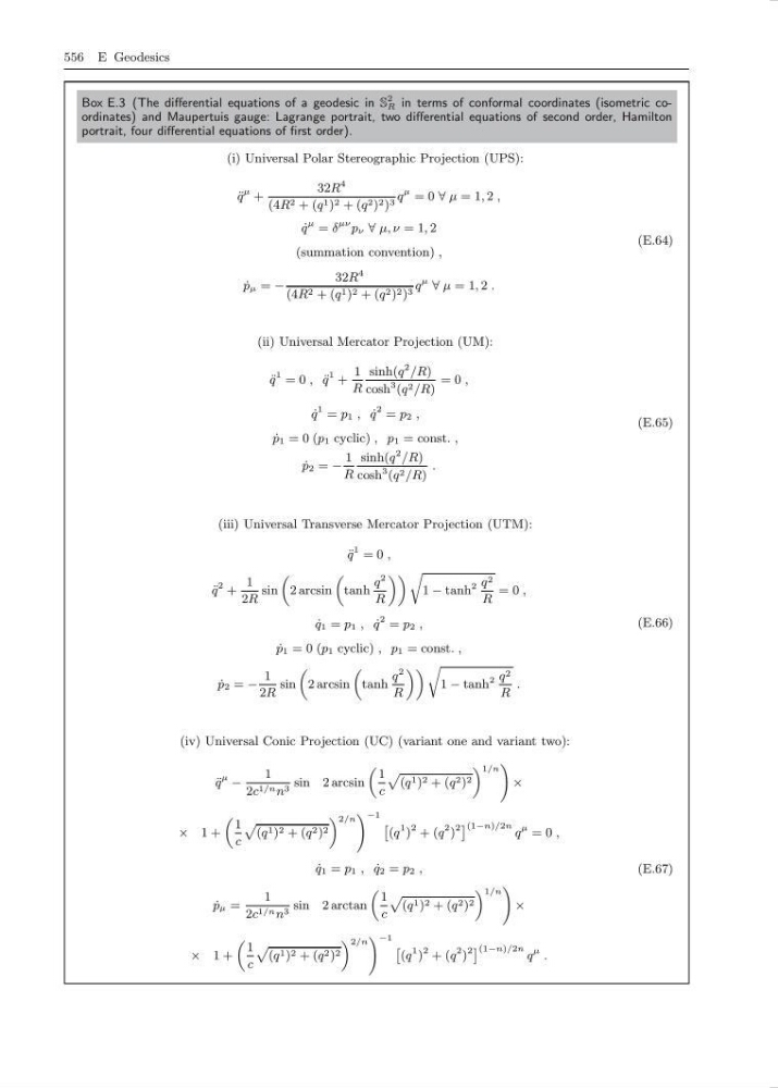
Box E.3 (The differential equations of a geodesic in S
2
R in terms of conformal coordinates (isometric coordinates) and Maupertuis gauge: Lagrange portrait, two differential equations of second order, Hamilton
portrait, four differential equations of first order).
(i) Universal Polar Stereographic Projection (UPS):
¨
q
µ +
32R
4
(4R 2 + (q 1 ) 2 + (q 2 ) 2 ) 3 q
µ = 0 ∀ µ = 1, 2 ,
˙
q
µ = δ
µν p ν ∀ µ, ν = 1, 2
(summation convention) ,
˙
p µ = −
32R
4
(4R 2 + (q 1 ) 2 + (q 2 ) 2 ) 3 q
µ ∀ µ = 1, 2 .
(E.64)
(ii) Universal Mercator Projection (UM):
¨
q
1 = 0 , ¨
q
1 +
1
R
sinh(q
2 /R)
cosh
3 (q 2 /R)
= 0 ,
˙
q
1 = p 1 , ˙
q
2 = p 2 ,
˙
p 1 = 0 (p 1 cyclic) , p 1 = const. ,
˙
p 2 = −
1
R
sinh(q
2 /R)
cosh
3 (q 2 /R)
.
(E.65)
(iii) Universal Transverse Mercator Projection (UTM):
¨
q
1 = 0 ,
¨
q
2 +
1
2R
sin
„
2 arcsin
„
tanh
q
2
R
«« r
1 − tanh
2 q 2
R
= 0 ,
˙
q 1 = p 1 , ˙
q
2 = p 2 ,
˙
p 1 = 0 (p 1 cyclic) , p 1 = const. ,
˙
p 2 = −
1
2R
sin
„
2 arcsin
„
tanh
q
2
R
«« r
1 − tanh
2 q 2
R
.
(E.66)
(iv) Universal Conic Projection (UC) (variant one and variant two):
¨
q
µ −
1
2c 1/n n 3 sin 2 arcsin
„
1
c
p
(q 1 ) 2 + (q 2 ) 2
« 1/n
!
×
× 1 +
„
1
c
p
(q 1 ) 2 + (q 2 ) 2
« 2/n
! −1 ˆ
(q
1 )
2 + (q
2 )
2 ˜ (1−n)/2n q
µ = 0 ,
˙
q 1 = p 1 , ˙
q 2 = p 2 ,
˙
p µ =
1
2c 1/n n 3 sin 2 arctan
„
1
c
p
(q 1 ) 2 + (q 2 ) 2
« 1/n
!
×
× 1 +
„
1
c
p
(q 1 ) 2 + (q 2 ) 2
« 2/n
! −1 ˆ
(q
1 )
2 + (q
2 )
2 ˜ (1−n)/2n q
µ .
(E.67)