

C-2 Elliptic kernel, elliptic modulus, elliptic functions, elliptic integrals 523
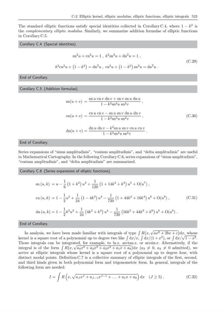
The standard elliptic functions satisfy special identities collected in Corollary C.4, where 1 − k
2 is
the complementary elliptic modulus. Similarly, we summarize addition formulae of elliptic functions
in Corollary C.5.
Corollary C.4 (Special identities).
sn
2 u + cn
2 u = 1 , k
2 sn
2 u + dn
2 u = 1 ,
k
2 cn
2 u +
1 − k
2
= dn
2 u , cn
2 u +
1 − k
2
sn
2 u = dn
2 u .
(C.29)
End of Corollary.
Corollary C.5 (Addition formulae).
sn(u + v) =
sn u cn v dn v + sn v sn u dn u
1 − k 2 sn 2 u sn 2 v
,
cn(u + v) =
cn u cn v − sn u sn v dn u dn v
1 − k 2 sn 2 u sn 2 v
,
dn(u + v) =
dn u dn v − k
2 sn u sn v cn u cn v
1 − k 2 sn 2 u sn 2 v
.
(C.30)
End of Corollary.
Series expansions of “sinus amplitudinis”, “cosinus amplitudinis”, and “delta amplitudinis” are useful
in Mathematical Cartography. In the following Corollary C.6, series expansions of “sinus amplitudinis”,
“cosinus amplitudinis”, and “delta amplitudinis” are summarized.
Corollary C.6 (Series expansions of elliptic functions).
sn (u, k) = u −
1
6
1 + k
2
u
3 +
1
120
1 + 14k
2 + k
4
u
5 + O(u
7 ) ,
cn (u, k) = 1 −
1
2
u
2 +
1
24
1 − 4k
2
u
4
−
1
720
1 + 44k
2 + 16k
4
u
6 + O(u
8 ) ,
dn (u, k) = 1 −
1
2
k
2 u
2 +
1
24
4k
2 + k
4
u
4
−
1
720
16k
2 + 44k
3 + k
6
u
6 + O(u
8 ) .
(C.31)
End of Corollary.
In analysis, we have been made familiar with integrals of type
R
x,
√
ax 2 + 2bx + c
dx, whose
kernel is a square root of a polynomial up to degree two like
dx/x,
dx/(1 + x
2 ), or
dx/
√
1 − x 2 .
Those integrals can be integrated, for example, to ln x, arctan x, or arcsin x. Alternatively, if the
integral is of the form
R
x,
√
a 4 x 4 + a 3 x 3 + a 2 x 2 + a 1 x + a 0
dx (a 3 = 0, a 4 = 0 admitted), we
arrive at elliptic integrals whose kernel is a square root of a polynomial up to degree four, with
distinct modal points. Definition C.7 is a collective summary of elliptic integrals of the first, second,
and third kinds given in both polynomial form and trigonometric form. In general, integrals of the
following form are needed:
I =
R
x,
a J x J + a J−1 x J−1 + . . . + a 1 x + a 0
dx (J ≥ 5) .
(C.32)
The standard elliptic functions satisfy special identities collected in Corollary C.4, where 1 − k
2 is
the complementary elliptic modulus. Similarly, we summarize addition formulae of elliptic functions
in Corollary C.5.
Corollary C.4 (Special identities).
sn
2 u + cn
2 u = 1 , k
2 sn
2 u + dn
2 u = 1 ,
k
2 cn
2 u +
1 − k
2
= dn
2 u , cn
2 u +
1 − k
2
sn
2 u = dn
2 u .
(C.29)
End of Corollary.
Corollary C.5 (Addition formulae).
sn(u + v) =
sn u cn v dn v + sn v sn u dn u
1 − k 2 sn 2 u sn 2 v
,
cn(u + v) =
cn u cn v − sn u sn v dn u dn v
1 − k 2 sn 2 u sn 2 v
,
dn(u + v) =
dn u dn v − k
2 sn u sn v cn u cn v
1 − k 2 sn 2 u sn 2 v
.
(C.30)
End of Corollary.
Series expansions of “sinus amplitudinis”, “cosinus amplitudinis”, and “delta amplitudinis” are useful
in Mathematical Cartography. In the following Corollary C.6, series expansions of “sinus amplitudinis”,
“cosinus amplitudinis”, and “delta amplitudinis” are summarized.
Corollary C.6 (Series expansions of elliptic functions).
sn (u, k) = u −
1
6
1 + k
2
u
3 +
1
120
1 + 14k
2 + k
4
u
5 + O(u
7 ) ,
cn (u, k) = 1 −
1
2
u
2 +
1
24
1 − 4k
2
u
4
−
1
720
1 + 44k
2 + 16k
4
u
6 + O(u
8 ) ,
dn (u, k) = 1 −
1
2
k
2 u
2 +
1
24
4k
2 + k
4
u
4
−
1
720
16k
2 + 44k
3 + k
6
u
6 + O(u
8 ) .
(C.31)
End of Corollary.
In analysis, we have been made familiar with integrals of type
R
x,
√
ax 2 + 2bx + c
dx, whose
kernel is a square root of a polynomial up to degree two like
dx/x,
dx/(1 + x
2 ), or
dx/
√
1 − x 2 .
Those integrals can be integrated, for example, to ln x, arctan x, or arcsin x. Alternatively, if the
integral is of the form
R
x,
√
a 4 x 4 + a 3 x 3 + a 2 x 2 + a 1 x + a 0
dx (a 3 = 0, a 4 = 0 admitted), we
arrive at elliptic integrals whose kernel is a square root of a polynomial up to degree four, with
distinct modal points. Definition C.7 is a collective summary of elliptic integrals of the first, second,
and third kinds given in both polynomial form and trigonometric form. In general, integrals of the
following form are needed:
I =
R
x,
a J x J + a J−1 x J−1 + . . . + a 1 x + a 0
dx (J ≥ 5) .
(C.32)