

B-3 Inversion of a multivariate homogeneous polynomial of degree n 517
Box B.3 (Algorithm for the construction of a multivariate homogeneous polynomial of degree n).
1st polynomial:
x =
n
X
k 1 =1
B 1k 1
0
@
n
X
k 2 =1
A 1k 2 x
[k 2 ]
1
A
[k 1 ]
+ β
1n+1 .
(B.61)
2nd polynomial:
x
[2] =
n
X
k=2
B 2k y
[k] + β
2n+1 =
n
X
k 1 =2
B 2k 1
0
@
n
X
k 2 =1
A 1k 2 x
[k 2 ]
1
A
[k 1 ]
+ β
2n+1 .
(B.62)
nth polynomial:
x
[n] = B nn y
[n] + β
nn+1 = B nn A nn x
[n] + β
nn+1 .
(B.63)
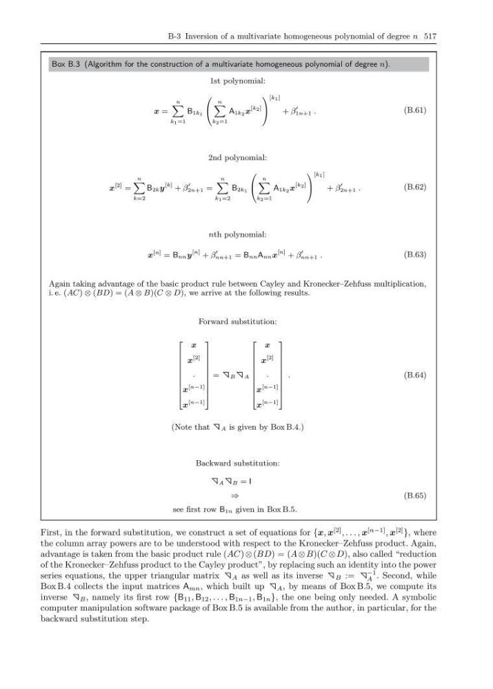
Again taking advantage of the basic product rule between Cayley and Kronecker–Zehfuss multiplication,
i. e. (AC) ⊗ (BD) = (A ⊗ B)(C ⊗ D), we arrive at the following results.
Forward substitution:
2
6
6
6
6
6
6
6
6
4
x
x
[2]
.
x
[n−1]
x
[n−1]
3
7
7
7
7
7
7
7
7
5
= B A
2
6
6
6
6
6
6
6
6
4
x
x
[2]
.
x
[n−1]
x
[n−1]
3
7
7
7
7
7
7
7
7
5
.
(B.64)
(Note that A is given by Box B.4.)
Backward substitution:
A
B = I
⇒
see first row B 1n given in Box B.5.
(B.65)
First, in the forward substitution, we construct a set of equations for {x, x
[2] , . . . , x
[n−1] , x
[2]
}, where
the column array powers are to be understood with respect to the Kronecker–Zehfuss product. Again,
advantage is taken from the basic product rule (AC) ⊗ (BD) = (A ⊗ B)(C ⊗ D), also called “reduction
of the Kronecker–Zehfuss product to the Cayley product”, by replacing such an identity into the power
series equations, the upper triangular matrix A as well as its inverse B :=
−1
A . Second, while
Box B.4 collects the input matrices A mn , which built up A , by means of Box B.5, we compute its
inverse B , namely its first row {B 11 , B 12 , . . . , B 1n−1 , B 1n }, the one being only needed. A symbolic
computer manipulation software package of Box B.5 is available from the author, in particular, for the
backward substitution step.
Box B.3 (Algorithm for the construction of a multivariate homogeneous polynomial of degree n).
1st polynomial:
x =
n
X
k 1 =1
B 1k 1
0
@
n
X
k 2 =1
A 1k 2 x
[k 2 ]
1
A
[k 1 ]
+ β
1n+1 .
(B.61)
2nd polynomial:
x
[2] =
n
X
k=2
B 2k y
[k] + β
2n+1 =
n
X
k 1 =2
B 2k 1
0
@
n
X
k 2 =1
A 1k 2 x
[k 2 ]
1
A
[k 1 ]
+ β
2n+1 .
(B.62)
nth polynomial:
x
[n] = B nn y
[n] + β
nn+1 = B nn A nn x
[n] + β
nn+1 .
(B.63)
Again taking advantage of the basic product rule between Cayley and Kronecker–Zehfuss multiplication,
i. e. (AC) ⊗ (BD) = (A ⊗ B)(C ⊗ D), we arrive at the following results.
Forward substitution:
2
6
6
6
6
6
6
6
6
4
x
x
[2]
.
x
[n−1]
x
[n−1]
3
7
7
7
7
7
7
7
7
5
= B A
2
6
6
6
6
6
6
6
6
4
x
x
[2]
.
x
[n−1]
x
[n−1]
3
7
7
7
7
7
7
7
7
5
.
(B.64)
(Note that A is given by Box B.4.)
Backward substitution:
A
B = I
⇒
see first row B 1n given in Box B.5.
(B.65)
First, in the forward substitution, we construct a set of equations for {x, x
[2] , . . . , x
[n−1] , x
[2]
}, where
the column array powers are to be understood with respect to the Kronecker–Zehfuss product. Again,
advantage is taken from the basic product rule (AC) ⊗ (BD) = (A ⊗ B)(C ⊗ D), also called “reduction
of the Kronecker–Zehfuss product to the Cayley product”, by replacing such an identity into the power
series equations, the upper triangular matrix A as well as its inverse B :=
−1
A . Second, while
Box B.4 collects the input matrices A mn , which built up A , by means of Box B.5, we compute its
inverse B , namely its first row {B 11 , B 12 , . . . , B 1n−1 , B 1n }, the one being only needed. A symbolic
computer manipulation software package of Box B.5 is available from the author, in particular, for the
backward substitution step.