

516 B The inverse of a multivariate homogeneous polynomial
Backward substitution:
A B = I 14 ⇔
⎡
⎢
⎢
⎣
B 11 B 12 B 13
0 B 22 B 23
0
0 B 33
⎤
⎥
⎥
⎦
⎡
⎢
⎢
⎣
A 11 A 12 A 13
0 A 22 A 23
0
0 A 33
⎤
⎥
⎥
⎦ = I 14 ;
(B.57)
(i) B 11 A 11 = I 2
⇒
B 11 = A
−1
11 ;
(ii) B 12 A 12 + B 12 A 22 = 0
⇒
B 12 = −B 11 A 12 A
−1
22 = −A
−1
11 A 12 A
−1[2]
22
;
(iii) B 11 A 13 + B 12 A 23 + B 13 A 33 = 0
⇒
B 13 = − (B 11 A 13 + B 12 A 23 ) A
−1
33 =
= −A
−1
11 A 13 A
−1[3]
11
+ A
−1
11 A 12 A
−1[2]
11
(A 11 ⊗ A 12 + A 12 ⊗ A 11 ) A
−1[3]
11
= A
−1
11
−A 13 + A 12
A
−1
11 ⊗ A
−1
11
(A 11 ⊗ A 12 + A 12 ⊗ A 11 )
A
−1
11 ⊗ A
−1
11 ⊗ A
−1
11
.
(B.58)
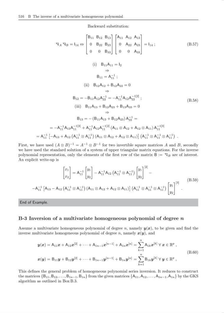
First, we have used (A ⊗ B)
−1 = A
−1
⊗ B
−1 for two invertible square matrices A and B, secondly
we have used the standard solution of a system of upper triangular matrix equations. For the inverse
polynomial representation, only the elements of the first row of the matrix B := B are of interest.
An explicit write-up is
x 1
x 2
= A
−1
11
y 1
y 2
− A
−1
11 A 12
A
−1
11 ⊗ A
−1
11
y 1
y 2
[2]
−
−A
−1
11
A 13 − A 12
A
−1
11 ⊗ A
−1
11
(A 11 ⊗ A 12 + A 12 ⊗ A 11 )
A
−1
11 ⊗ A
−1
11 ⊗ A
−1
11
y 1
y 2
[3]
.
(B.59)
End of Example.
B-3 Inversion of a multivariate homogeneous polynomial of degree n
Assume a multivariate homogeneous polynomial of degree n, namely y(x), to be given and find the
inverse multivariate homogeneous polynomial of degree n, namely x(y), and
y(x) = A 11 x + A 12 x
[2] + · · · + A 1n−1 x
[n−1] + A 1n x
[n] =
n
k=1
A 1k x
[k]
∀ x ∈ R
p ,
x(y) = B 11 y + B 12 y
[2] + · · · + B 1n−1 y
[n−1] + B 1n y
[n] =
n
k=1
B 1k y
[k]
∀ y ∈ R
p ,
(B.60)
This defines the general problem of homogeneous polynomial series inversion. It reduces to construct
the matrices {B 11 , B 12 , . . . , B 1n−1 , B 1n } from the given matrices {A 11 , A 12 , . . . , A 1n−1 , A 1n } by the GKS
algorithm as outlined in Box B.3.
Backward substitution:
A B = I 14 ⇔
⎡
⎢
⎢
⎣
B 11 B 12 B 13
0 B 22 B 23
0
0 B 33
⎤
⎥
⎥
⎦
⎡
⎢
⎢
⎣
A 11 A 12 A 13
0 A 22 A 23
0
0 A 33
⎤
⎥
⎥
⎦ = I 14 ;
(B.57)
(i) B 11 A 11 = I 2
⇒
B 11 = A
−1
11 ;
(ii) B 12 A 12 + B 12 A 22 = 0
⇒
B 12 = −B 11 A 12 A
−1
22 = −A
−1
11 A 12 A
−1[2]
22
;
(iii) B 11 A 13 + B 12 A 23 + B 13 A 33 = 0
⇒
B 13 = − (B 11 A 13 + B 12 A 23 ) A
−1
33 =
= −A
−1
11 A 13 A
−1[3]
11
+ A
−1
11 A 12 A
−1[2]
11
(A 11 ⊗ A 12 + A 12 ⊗ A 11 ) A
−1[3]
11
= A
−1
11
−A 13 + A 12
A
−1
11 ⊗ A
−1
11
(A 11 ⊗ A 12 + A 12 ⊗ A 11 )
A
−1
11 ⊗ A
−1
11 ⊗ A
−1
11
.
(B.58)
First, we have used (A ⊗ B)
−1 = A
−1
⊗ B
−1 for two invertible square matrices A and B, secondly
we have used the standard solution of a system of upper triangular matrix equations. For the inverse
polynomial representation, only the elements of the first row of the matrix B := B are of interest.
An explicit write-up is
x 1
x 2
= A
−1
11
y 1
y 2
− A
−1
11 A 12
A
−1
11 ⊗ A
−1
11
y 1
y 2
[2]
−
−A
−1
11
A 13 − A 12
A
−1
11 ⊗ A
−1
11
(A 11 ⊗ A 12 + A 12 ⊗ A 11 )
A
−1
11 ⊗ A
−1
11 ⊗ A
−1
11
y 1
y 2
[3]
.
(B.59)
End of Example.
B-3 Inversion of a multivariate homogeneous polynomial of degree n
Assume a multivariate homogeneous polynomial of degree n, namely y(x), to be given and find the
inverse multivariate homogeneous polynomial of degree n, namely x(y), and
y(x) = A 11 x + A 12 x
[2] + · · · + A 1n−1 x
[n−1] + A 1n x
[n] =
n
k=1
A 1k x
[k]
∀ x ∈ R
p ,
x(y) = B 11 y + B 12 y
[2] + · · · + B 1n−1 y
[n−1] + B 1n y
[n] =
n
k=1
B 1k y
[k]
∀ y ∈ R
p ,
(B.60)
This defines the general problem of homogeneous polynomial series inversion. It reduces to construct
the matrices {B 11 , B 12 , . . . , B 1n−1 , B 1n } from the given matrices {A 11 , A 12 , . . . , A 1n−1 , A 1n } by the GKS
algorithm as outlined in Box B.3.