

34
1 From Riemann manifolds to Riemann manifolds
Solution (the first and the second problem).
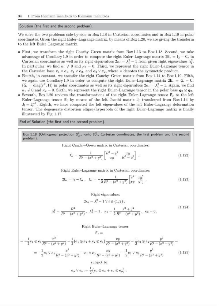
We solve the two problems side-by-side in Box 1.18 in Cartesian coordinates and in Box 1.19 in polar
coordinates. Given the right Euler–Lagrange matrix, by means of Box 1.20, we are giving the transform
to the left Euler–Lagrange matrix.
• First, we transform the right Cauchy–Green matrix from Box 1.13 to Box 1.18. Second, we take
advantage of Corollary 1.9 in order to compute the right Euler–Lagrange matrix 2E r = I 2 − C r in
Cartesian coordinates as well as its right eigenvalues 2κ i = λ
2
i − 1 from given right eigenvalues λ
2
i .
In particular, we find κ 1 = 0 and κ 2 = 0. Third, we represent the right Euler–Lagrange tensor in
the Cartesian base e 1 ∨ e 1 , e 1 ∨ e 2 , and e 2 ∨ e 2 , where ∨ denotes the symmetric product.
• Fourth, in contrast, we transfer the right Cauchy–Green matrix from Box 1.14 to Box 1.19. Fifth,
we again use Corollary 1.9 in order to compute the right Euler–Lagrange matrix 2E r = G r − C r
(G r = diag(r
2 , 1)) in polar coordinates as well as its right eigenvalues 2κ i = λ
2
i − 1. Again, we find
κ 1 = 0 and κ 2 = 0. Sixth, we represent the right Euler–Lagrange tensor in the polar base g 2 ⊗ g 2 .
• Seventh, Box 1.20 reviews the transformations of the right Euler–Lagrange tensor E r to the left
Euler–Lagrange tensor E l by means of the left Jacobi matrix J l transferred from Box 1.14 by
J l = J
−1
r . Eighth, we have computed the left eigenvalues of the left Euler–Lagrange deformation
tensor. The degenerate distortion ellipse/hyperbola of the right Euler–Lagrange matrix is finally
illustrated by Fig. 1.17.
End of Solution (the first and the second problem).
Box 1.18 (Orthogonal projection S
2
R + onto P
2
O , Cartesian coordinates, the first problem and the second
problem).
Right Cauchy–Green matrix in Cartesian coordinates:
C r =
1
R 2 − (x 2 + y 2 )
»
R
2 − y
2
xy
xy
R
2 − x
2
–
.
(1.122)
Right Euler–Lagrange matrix in Cartesian coordinates:
2E r = I 2 − C r , E r = −
1
2
1
R 2 − (x 2 + y 2 )
»
x
2
xy
xy y
2
–
.
(1.123)
Right eigenvalues:
2κ i = λ
2
i − 1 ∀ i ∈ {1, 2} ,
λ
2
1 =
R
2
R 2 − (x 2 + y 2 )
, λ
2
2 = 1 , κ 1 =
1
2
x
2 + y
2
R 2 − (x 2 + y 2 )
, κ 2 = 0 .
(1.124)
Right Euler–Lagrange tensor:
E r =
= −
1
2
e 1 ⊗ e 1
x
2
R 2 − (x 2 + y 2 )
−
1
2
`
e 1 ⊗ e 2 + e 2 ⊗ e 1
´
xy
R 2 − (x 2 + y 2 )
−
1
2
e 2 ⊗ e 2
y
2
R 2 − (x 2 + y 2 )
=
= −
1
2
e 1 ∨ e 1
x
2
R 2 − (x 2 + y 2 )
− e 1 ∨ e 2
xy
R 2 − (x 2 + y 2 )
−
1
2
e 2 ∨ e 2
y
2
R 2 − (x 2 + y 2 )
subject to
e µ ∨ e ν :=
1
2
`
e µ ⊗ e ν + e ν ⊗ e µ
´
.
(1.125)
1 From Riemann manifolds to Riemann manifolds
Solution (the first and the second problem).
We solve the two problems side-by-side in Box 1.18 in Cartesian coordinates and in Box 1.19 in polar
coordinates. Given the right Euler–Lagrange matrix, by means of Box 1.20, we are giving the transform
to the left Euler–Lagrange matrix.
• First, we transform the right Cauchy–Green matrix from Box 1.13 to Box 1.18. Second, we take
advantage of Corollary 1.9 in order to compute the right Euler–Lagrange matrix 2E r = I 2 − C r in
Cartesian coordinates as well as its right eigenvalues 2κ i = λ
2
i − 1 from given right eigenvalues λ
2
i .
In particular, we find κ 1 = 0 and κ 2 = 0. Third, we represent the right Euler–Lagrange tensor in
the Cartesian base e 1 ∨ e 1 , e 1 ∨ e 2 , and e 2 ∨ e 2 , where ∨ denotes the symmetric product.
• Fourth, in contrast, we transfer the right Cauchy–Green matrix from Box 1.14 to Box 1.19. Fifth,
we again use Corollary 1.9 in order to compute the right Euler–Lagrange matrix 2E r = G r − C r
(G r = diag(r
2 , 1)) in polar coordinates as well as its right eigenvalues 2κ i = λ
2
i − 1. Again, we find
κ 1 = 0 and κ 2 = 0. Sixth, we represent the right Euler–Lagrange tensor in the polar base g 2 ⊗ g 2 .
• Seventh, Box 1.20 reviews the transformations of the right Euler–Lagrange tensor E r to the left
Euler–Lagrange tensor E l by means of the left Jacobi matrix J l transferred from Box 1.14 by
J l = J
−1
r . Eighth, we have computed the left eigenvalues of the left Euler–Lagrange deformation
tensor. The degenerate distortion ellipse/hyperbola of the right Euler–Lagrange matrix is finally
illustrated by Fig. 1.17.
End of Solution (the first and the second problem).
Box 1.18 (Orthogonal projection S
2
R + onto P
2
O , Cartesian coordinates, the first problem and the second
problem).
Right Cauchy–Green matrix in Cartesian coordinates:
C r =
1
R 2 − (x 2 + y 2 )
»
R
2 − y
2
xy
xy
R
2 − x
2
–
.
(1.122)
Right Euler–Lagrange matrix in Cartesian coordinates:
2E r = I 2 − C r , E r = −
1
2
1
R 2 − (x 2 + y 2 )
»
x
2
xy
xy y
2
–
.
(1.123)
Right eigenvalues:
2κ i = λ
2
i − 1 ∀ i ∈ {1, 2} ,
λ
2
1 =
R
2
R 2 − (x 2 + y 2 )
, λ
2
2 = 1 , κ 1 =
1
2
x
2 + y
2
R 2 − (x 2 + y 2 )
, κ 2 = 0 .
(1.124)
Right Euler–Lagrange tensor:
E r =
= −
1
2
e 1 ⊗ e 1
x
2
R 2 − (x 2 + y 2 )
−
1
2
`
e 1 ⊗ e 2 + e 2 ⊗ e 1
´
xy
R 2 − (x 2 + y 2 )
−
1
2
e 2 ⊗ e 2
y
2
R 2 − (x 2 + y 2 )
=
= −
1
2
e 1 ∨ e 1
x
2
R 2 − (x 2 + y 2 )
− e 1 ∨ e 2
xy
R 2 − (x 2 + y 2 )
−
1
2
e 2 ∨ e 2
y
2
R 2 − (x 2 + y 2 )
subject to
e µ ∨ e ν :=
1
2
`
e µ ⊗ e ν + e ν ⊗ e µ
´
.
(1.125)