

21-4 Gauss–Krueger/UTM coordinates: from a local to a global datum 485
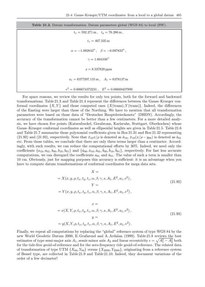
Table 21.2. Datum transformation. Datum parameters global (WGS 84) to local (BW).
t x = 592.271 m , t y = 76.286 m ,
t z = 407.335 m
α = −1.092843
, β = −0.097832
,
γ = 1.604106
s = 8.537829 ppm
a 1 = 6377397.155 m , A 1 = 6378137 m
e
2 = 0.006674372231 , E
2 = 0.00669437999
For space reasons, we review the results for only ten points, both for the forward and backward
transformations. Table 21.3 and Table 21.4 represent the differences between the Gauss–Krueger conformal coordinates {X, Y } and those computed ones {X(trans), Y (trans)}. Indeed, the differences
of the Easting were larger than those of the Northing. We have to mention that all transformation
parameters were based on those data of “Deutsches Hauptdreiecksnetz” (DHDN). Accordingly, the
accuracy of the transformation cannot be better than a few centimeters. For a more detailed analysis, we have chosen five points (Katzenbuckel, Gerabronn, Karlsruhe, Stuttgart, Oberkochen) whose
Gauss–Krueger conformal coordinates as well as ellipsoidal heights are given in Table 21.5. Table 21.6
and Table 21.7 summarize those polynomial coefficients given in Box 21.31 and Box 21.32 representing
(21.92) and (21.93), respectively. Note that ¯
x 10 x/ρ is denoted as ¯
a 10 , ¯
x 10 (x/ρ − y 00 ) is denoted as ¯
a 01
etc. From those tables, we conclude that there are only three terms larger than a centimeter. Accordingly, with such results, we can reduce the computational efforts by 30%. Indeed, we need only the
coefficients {a 10 , a 01 , b 00 , b 10 , b 01 } and {¯ a 00 , ¯
a 10 , ¯
a 01 , ¯ b 00 , ¯ b 10 , ¯ b 01 }, respectively. For fast less accurate
computations, we can disregard the coefficients a 01 and ¯
a 01 . The value of such a term is smaller than
10 cm. Obviously, just for mapping purposes this accuracy is sufficient: it is an advantage when you
have to compute datum transformations of conformal coordinates for mega data sets.
X =
= X(x, y, ρ, t x , t y , t z , α, β, γ, s, A 1 , E
2 , a 1 , e
2 ) ,
Y =
= Y (x, y, ρ, t x , t y , t z , α, β, γ, s, A 1 , E
2 , a 1 , e
2 ) ,
(21.92)
x =
= x(X, Y, ρ, t x , t y , t z , α, β, γ, s, A 1 , E
2 , a 1 , e
2 ) ,
y =
= y(X, Y, ρ, t x , t y , t z , α, β, γ, s, A 1 , E
2 , a 1 , e
2 ) .
(21.93)
Finally, we repeat all computations by replacing the “global” reference system of type WGS 84 by the
new World Geodetic Datum 2000, E. Grafarend and A. Ardalan (1999). Table 21.8 reviews the best
estimates of type semi-major axis A 1 , semir-minor axis A 2 and linear eccentricity =
A 2
1 − A 2
2 both
for the tide-free geoid-of-reference and for the zero-frequency tide geoid-of-reference. The related data
of transformation of type UTM {X 84 , Y 84 } versus {X 2000 , Y 2000 }, originating from a reference system
of Bessel type, are collected in Table 21.9 and Table 21.10. Indeed, they document variations of the
order of a few decimeter!
Table 21.2. Datum transformation. Datum parameters global (WGS 84) to local (BW).
t x = 592.271 m , t y = 76.286 m ,
t z = 407.335 m
α = −1.092843
, β = −0.097832
,
γ = 1.604106
s = 8.537829 ppm
a 1 = 6377397.155 m , A 1 = 6378137 m
e
2 = 0.006674372231 , E
2 = 0.00669437999
For space reasons, we review the results for only ten points, both for the forward and backward
transformations. Table 21.3 and Table 21.4 represent the differences between the Gauss–Krueger conformal coordinates {X, Y } and those computed ones {X(trans), Y (trans)}. Indeed, the differences
of the Easting were larger than those of the Northing. We have to mention that all transformation
parameters were based on those data of “Deutsches Hauptdreiecksnetz” (DHDN). Accordingly, the
accuracy of the transformation cannot be better than a few centimeters. For a more detailed analysis, we have chosen five points (Katzenbuckel, Gerabronn, Karlsruhe, Stuttgart, Oberkochen) whose
Gauss–Krueger conformal coordinates as well as ellipsoidal heights are given in Table 21.5. Table 21.6
and Table 21.7 summarize those polynomial coefficients given in Box 21.31 and Box 21.32 representing
(21.92) and (21.93), respectively. Note that ¯
x 10 x/ρ is denoted as ¯
a 10 , ¯
x 10 (x/ρ − y 00 ) is denoted as ¯
a 01
etc. From those tables, we conclude that there are only three terms larger than a centimeter. Accordingly, with such results, we can reduce the computational efforts by 30%. Indeed, we need only the
coefficients {a 10 , a 01 , b 00 , b 10 , b 01 } and {¯ a 00 , ¯
a 10 , ¯
a 01 , ¯ b 00 , ¯ b 10 , ¯ b 01 }, respectively. For fast less accurate
computations, we can disregard the coefficients a 01 and ¯
a 01 . The value of such a term is smaller than
10 cm. Obviously, just for mapping purposes this accuracy is sufficient: it is an advantage when you
have to compute datum transformations of conformal coordinates for mega data sets.
X =
= X(x, y, ρ, t x , t y , t z , α, β, γ, s, A 1 , E
2 , a 1 , e
2 ) ,
Y =
= Y (x, y, ρ, t x , t y , t z , α, β, γ, s, A 1 , E
2 , a 1 , e
2 ) ,
(21.92)
x =
= x(X, Y, ρ, t x , t y , t z , α, β, γ, s, A 1 , E
2 , a 1 , e
2 ) ,
y =
= y(X, Y, ρ, t x , t y , t z , α, β, γ, s, A 1 , E
2 , a 1 , e
2 ) .
(21.93)
Finally, we repeat all computations by replacing the “global” reference system of type WGS 84 by the
new World Geodetic Datum 2000, E. Grafarend and A. Ardalan (1999). Table 21.8 reviews the best
estimates of type semi-major axis A 1 , semir-minor axis A 2 and linear eccentricity =
A 2
1 − A 2
2 both
for the tide-free geoid-of-reference and for the zero-frequency tide geoid-of-reference. The related data
of transformation of type UTM {X 84 , Y 84 } versus {X 2000 , Y 2000 }, originating from a reference system
of Bessel type, are collected in Table 21.9 and Table 21.10. Indeed, they document variations of the
order of a few decimeter!