

478 21 Datum problems
{m, n} ↔ l mn
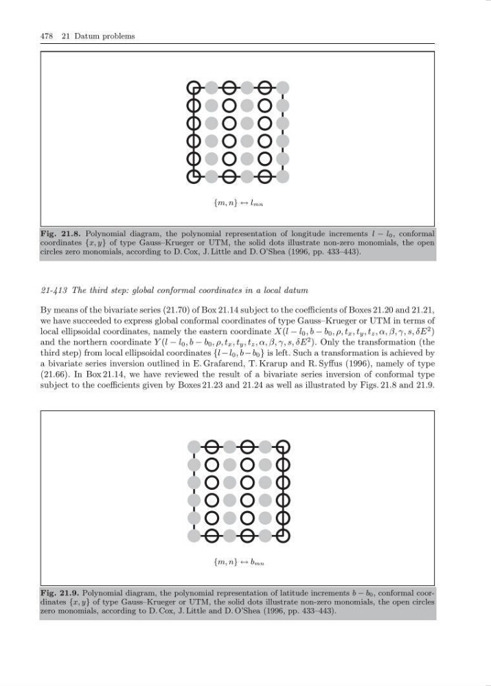
Fig. 21.8. Polynomial diagram, the polynomial representation of longitude increments l − l 0 , conformal
coordinates {x, y} of type Gauss–Krueger or UTM, the solid dots illustrate non-zero monomials, the open
circles zero monomials, according to D. Cox, J. Little and D. O’Shea (1996, pp. 433–443).
21-413 The third step: global conformal coordinates in a local datum
By means of the bivariate series (21.70) of Box 21.14 subject to the coefficients of Boxes 21.20 and 21.21,
we have succeeded to express global conformal coordinates of type Gauss–Krueger or UTM in terms of
local ellipsoidal coordinates, namely the eastern coordinate X(l − l 0 , b − b 0 , ρ, t x , t y , t z , α, β, γ, s, δE
2 )
and the northern coordinate Y (l − l 0 , b − b 0 , ρ, t x , t y , t z , α, β, γ, s, δE
2 ). Only the transformation (the
third step) from local ellipsoidal coordinates {l −l 0 , b−b 0 } is left. Such a transformation is achieved by
a bivariate series inversion outlined in E. Grafarend, T. Krarup and R. Syffus (1996), namely of type
(21.66). In Box 21.14, we have reviewed the result of a bivariate series inversion of conformal type
subject to the coefficients given by Boxes 21.23 and 21.24 as well as illustrated by Figs. 21.8 and 21.9.
{m, n} ↔ b mn
Fig. 21.9. Polynomial diagram, the polynomial representation of latitude increments b − b 0 , conformal coordinates {x, y} of type Gauss–Krueger or UTM, the solid dots illustrate non-zero monomials, the open circles
zero monomials, according to D. Cox, J. Little and D. O’Shea (1996, pp. 433–443).
{m, n} ↔ l mn
Fig. 21.8. Polynomial diagram, the polynomial representation of longitude increments l − l 0 , conformal
coordinates {x, y} of type Gauss–Krueger or UTM, the solid dots illustrate non-zero monomials, the open
circles zero monomials, according to D. Cox, J. Little and D. O’Shea (1996, pp. 433–443).
21-413 The third step: global conformal coordinates in a local datum
By means of the bivariate series (21.70) of Box 21.14 subject to the coefficients of Boxes 21.20 and 21.21,
we have succeeded to express global conformal coordinates of type Gauss–Krueger or UTM in terms of
local ellipsoidal coordinates, namely the eastern coordinate X(l − l 0 , b − b 0 , ρ, t x , t y , t z , α, β, γ, s, δE
2 )
and the northern coordinate Y (l − l 0 , b − b 0 , ρ, t x , t y , t z , α, β, γ, s, δE
2 ). Only the transformation (the
third step) from local ellipsoidal coordinates {l −l 0 , b−b 0 } is left. Such a transformation is achieved by
a bivariate series inversion outlined in E. Grafarend, T. Krarup and R. Syffus (1996), namely of type
(21.66). In Box 21.14, we have reviewed the result of a bivariate series inversion of conformal type
subject to the coefficients given by Boxes 21.23 and 21.24 as well as illustrated by Figs. 21.8 and 21.9.
{m, n} ↔ b mn
Fig. 21.9. Polynomial diagram, the polynomial representation of latitude increments b − b 0 , conformal coordinates {x, y} of type Gauss–Krueger or UTM, the solid dots illustrate non-zero monomials, the open circles
zero monomials, according to D. Cox, J. Little and D. O’Shea (1996, pp. 433–443).