

21-4 Gauss–Krueger/ UTM coordinates:from a local to a global datum 471
curv ilinear
datum transformation
step tw o
1
step three
2
step tw o
2
step three
1
step one
{x, y}, E
2
a 1 ,a 2
{X, Y }, E
2
A 1 ,A 2
{L − L 0 , B − B 0 }
{ l − l 0 , b − b 0 }
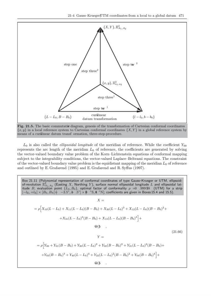
Fig. 21.5. The basic commutativ e diagram, genesis of the transformation of Cartesian conformal coordinates
{x, y} in a local reference system to Cartesian conformal coordinates {X, Y } in a global reference system by
means of a curv ilinear datum transf ormation, three-step-procedure.
L 0 is also called the ellipsoidal longitude of the meridian of reference. While the coefficient Y 00
represents the arc length of the meridian L 0 of reference, the coefficients are generated by solving
the vector-valued boundary value problem of the Korn–Lichtenstein equations of conformal mapping
subject to the integrability conditions, the vector-valued Laplace–Beltrami equations. The constraint
of the vector-valued boundary value problem is the equidistant mapping of the meridian L 0 of reference
and outlined by E. Grafarend (1995) and E. Grafarend and R. Syffus (1997).
Box 21.11 (Polynomial representation of conformal coordinates of type Gauss–Krueger or UTM, ellipsoidof-revolution E
2
A 1 ,A 2 (Easting X, Northing Y ), surface normal ellipsoidal longitude L and ellipsoidal latitude B, evaluation point {L 0 , B 0 }, optimal factor of conformality ρ =0 .999 5
78 (UTM) for a strip
[−l E , +l E ] × [B S , B N ]= [ −3.5
◦ , +
3 .5
◦ ] × [
8
0
◦ S, 8
4
◦ N]; coefficients are given in Boxes 15.4 and 15.5).
X =
= ρ
h
X 10 (L − L 0 ) + X 11 (L − L 0 )(B − B 0 ) + X 30 (L − L 0 )
3 + X 12 (L − L 0 )(B − B 0 )
2 +
+X 31 (L − L 0 )
3 (B − B 0 ) + X 13 (L − L 0 )(B − B 0 )
3
i
+
+
O(5 )
,
Y =
= ρ
h
Y 00 + Y 01 (B − B 0 ) + Y 20 (L − L 0 )
2 + Y 02 (B − B 0 )
2 + Y 21 (L − L 0 )
2 (B − B 0 )+
+Y 03 (B − B 0 )
3 + Y 40 (L − L 0 )
4 + Y 22 (L − L 0 )
2 (B − B 0 )
2 + Y 04 (B − B 0 )
4
i
+
+
O(5 )
.
(21.66)
curv ilinear
datum transformation
step tw o
1
step three
2
step tw o
2
step three
1
step one
{x, y}, E
2
a 1 ,a 2
{X, Y }, E
2
A 1 ,A 2
{L − L 0 , B − B 0 }
{ l − l 0 , b − b 0 }
Fig. 21.5. The basic commutativ e diagram, genesis of the transformation of Cartesian conformal coordinates
{x, y} in a local reference system to Cartesian conformal coordinates {X, Y } in a global reference system by
means of a curv ilinear datum transf ormation, three-step-procedure.
L 0 is also called the ellipsoidal longitude of the meridian of reference. While the coefficient Y 00
represents the arc length of the meridian L 0 of reference, the coefficients are generated by solving
the vector-valued boundary value problem of the Korn–Lichtenstein equations of conformal mapping
subject to the integrability conditions, the vector-valued Laplace–Beltrami equations. The constraint
of the vector-valued boundary value problem is the equidistant mapping of the meridian L 0 of reference
and outlined by E. Grafarend (1995) and E. Grafarend and R. Syffus (1997).
Box 21.11 (Polynomial representation of conformal coordinates of type Gauss–Krueger or UTM, ellipsoidof-revolution E
2
A 1 ,A 2 (Easting X, Northing Y ), surface normal ellipsoidal longitude L and ellipsoidal latitude B, evaluation point {L 0 , B 0 }, optimal factor of conformality ρ =0 .999 5
78 (UTM) for a strip
[−l E , +l E ] × [B S , B N ]= [ −3.5
◦ , +
3 .5
◦ ] × [
8
0
◦ S, 8
4
◦ N]; coefficients are given in Boxes 15.4 and 15.5).
X =
= ρ
h
X 10 (L − L 0 ) + X 11 (L − L 0 )(B − B 0 ) + X 30 (L − L 0 )
3 + X 12 (L − L 0 )(B − B 0 )
2 +
+X 31 (L − L 0 )
3 (B − B 0 ) + X 13 (L − L 0 )(B − B 0 )
3
i
+
+
O(5 )
,
Y =
= ρ
h
Y 00 + Y 01 (B − B 0 ) + Y 20 (L − L 0 )
2 + Y 02 (B − B 0 )
2 + Y 21 (L − L 0 )
2 (B − B 0 )+
+Y 03 (B − B 0 )
3 + Y 40 (L − L 0 )
4 + Y 22 (L − L 0 )
2 (B − B 0 )
2 + Y 04 (B − B 0 )
4
i
+
+
O(5 )
.
(21.66)