

20-5 Deformation analysis: Riemann, Soldner, Gauss–Krueger coordinates 451
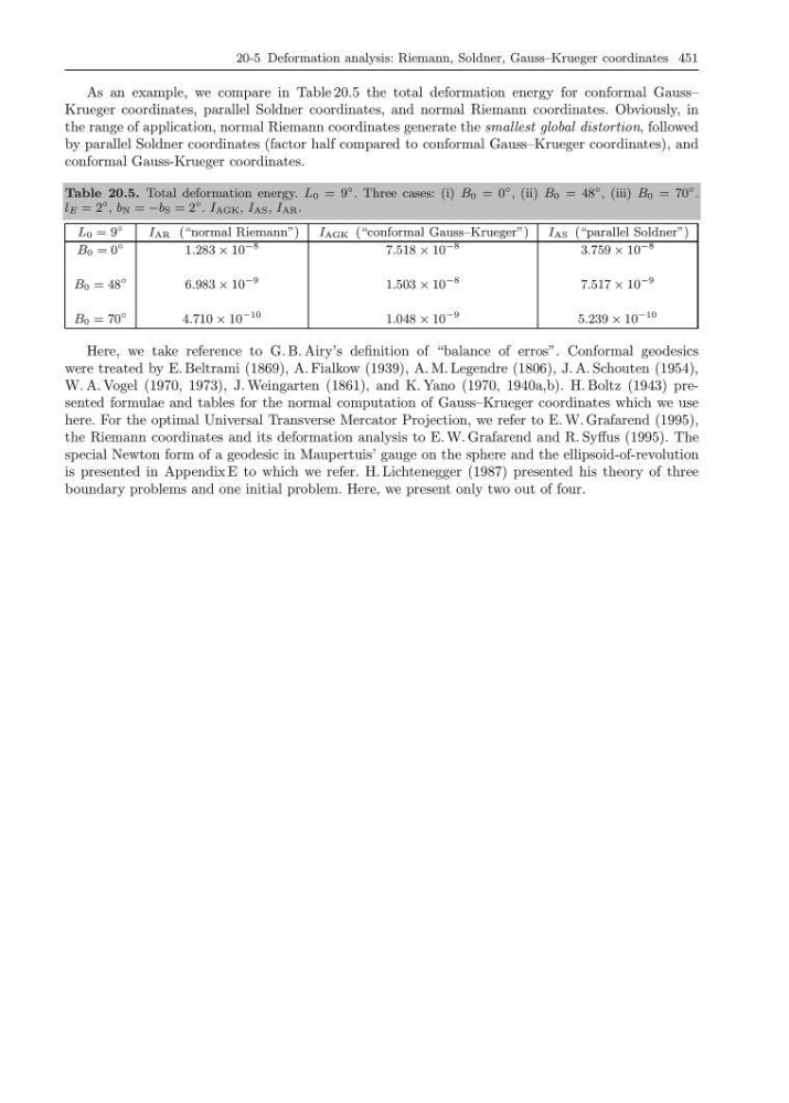
As an example, we compare in Table 20.5 the total deformation energy for conformal Gauss–
Krueger coordinates, parallel Soldner coordinates, and normal Riemann coordinates. Obviously, in
the range of application, normal Riemann coordinates generate the smallest global distortion, followed
by parallel Soldner coordinates (factor half compared to conformal Gauss–Krueger coordinates), and
conformal Gauss-Krueger coordinates.
Table 20.5. Total deformation energy. L 0 = 9
◦ . Three cases: (i) B 0 = 0
◦ , (ii) B 0 = 48
◦ , (iii) B 0 = 70
◦ .
l E = 2
◦ , b N = −b S = 2
◦ . I AGK , I AS , I AR .
L 0 = 9
◦
I AR (“normal Riemann”)
I AGK (“conformal Gauss–Krueger”) I AS (“parallel Soldner”)
B 0 = 0
◦
1.283 × 10
−8
7.518 × 10
−8
3.759 × 10
−8
B 0 = 48
◦
6.983 × 10
−9
1.503 × 10
−8
7.517 × 10
−9
B 0 = 70
◦
4.710 × 10
−10
1.048 × 10
−9
5.239 × 10
−10
Here, we take reference to G. B. Airy’s definition of “balance of erros”. Conformal geodesics
were treated by E. Beltrami (1869), A. Fialkow (1939), A. M. Legendre (1806), J. A. Schouten (1954),
W. A. Vogel (1970, 1973), J. Weingarten (1861), and K. Yano (1970, 1940a,b). H. Boltz (1943) presented formulae and tables for the normal computation of Gauss–Krueger coordinates which we use
here. For the optimal Universal Transverse Mercator Projection, we refer to E. W. Grafarend (1995),
the Riemann coordinates and its deformation analysis to E. W. Grafarend and R. Syffus (1995). The
special Newton form of a geodesic in Maupertuis’ gauge on the sphere and the ellipsoid-of-revolution
is presented in Appendix E to which we refer. H. Lichtenegger (1987) presented his theory of three
boundary problems and one initial problem. Here, we present only two out of four.
As an example, we compare in Table 20.5 the total deformation energy for conformal Gauss–
Krueger coordinates, parallel Soldner coordinates, and normal Riemann coordinates. Obviously, in
the range of application, normal Riemann coordinates generate the smallest global distortion, followed
by parallel Soldner coordinates (factor half compared to conformal Gauss–Krueger coordinates), and
conformal Gauss-Krueger coordinates.
Table 20.5. Total deformation energy. L 0 = 9
◦ . Three cases: (i) B 0 = 0
◦ , (ii) B 0 = 48
◦ , (iii) B 0 = 70
◦ .
l E = 2
◦ , b N = −b S = 2
◦ . I AGK , I AS , I AR .
L 0 = 9
◦
I AR (“normal Riemann”)
I AGK (“conformal Gauss–Krueger”) I AS (“parallel Soldner”)
B 0 = 0
◦
1.283 × 10
−8
7.518 × 10
−8
3.759 × 10
−8
B 0 = 48
◦
6.983 × 10
−9
1.503 × 10
−8
7.517 × 10
−9
B 0 = 70
◦
4.710 × 10
−10
1.048 × 10
−9
5.239 × 10
−10
Here, we take reference to G. B. Airy’s definition of “balance of erros”. Conformal geodesics
were treated by E. Beltrami (1869), A. Fialkow (1939), A. M. Legendre (1806), J. A. Schouten (1954),
W. A. Vogel (1970, 1973), J. Weingarten (1861), and K. Yano (1970, 1940a,b). H. Boltz (1943) presented formulae and tables for the normal computation of Gauss–Krueger coordinates which we use
here. For the optimal Universal Transverse Mercator Projection, we refer to E. W. Grafarend (1995),
the Riemann coordinates and its deformation analysis to E. W. Grafarend and R. Syffus (1995). The
special Newton form of a geodesic in Maupertuis’ gauge on the sphere and the ellipsoid-of-revolution
is presented in Appendix E to which we refer. H. Lichtenegger (1987) presented his theory of three
boundary problems and one initial problem. Here, we present only two out of four.