

434 20 Geodetic mapping
The construction principle is as follows. A point P 0 (L 0 , B 0 ) is defined as the origin of a local reference
system. The x c axis of the coordinate system, which is called “Hochwert” (Soldner wording), agrees
with the chosen reference meridian L 0 . A point P (L, B) is described by geodetic parallel coordinates
as follows. Through the point P , we compute the unique geodetic line, which cuts the meridian L 0 at
a right angle to produce the footprint point P F . The length of the geodesic P –P F is chosen as the y c
coordinate, which is called “Rechtswert” (Soldner wording). The angle which is in between the local
meridian of the point P and the geodetic parallel through the point P is called meridian convergence
γ = A PF − π/2. The angle γ is fixed as the northern part of the meridian, lefthand-oriented positive.
We always say that the azimuth of the coordinate line y c = const. is the angle γ. Most notable, the
geodetic parallel y c = const. is not a geodesic. Compare with Fig. 20.4.
Important!
The y c lines produce the geodesic field. In contrast, the geodetic parallels are the orthogonal
trajectories ds
2 = E(x c , y c )dx
2
c + dy
2
c = dx
2 + G(x, y)dy
2 .
20-31 First problem of Soldner coordinates: geodetic parallel coordinates, input
{L 0 , B 0 , x c = y, y c = x} versus output {L, B, γ (meridian convergence)}
For the problem of given coordinates {L 0 , B 0 , x c = y, y c = x} and unknown coordinates {L, B, γ}, we
use the standard method of Legendre series u = s cos α 0P and v = s sin α 0P . In Box 20.7, the details
are collected.
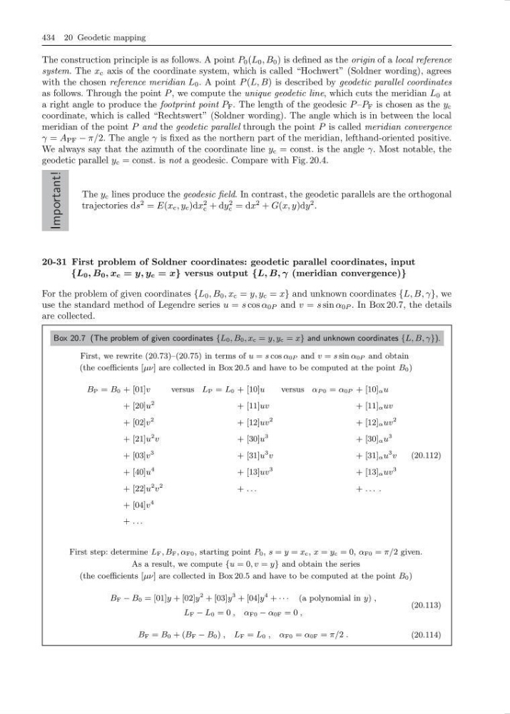
Box 20.7 (The problem of given coordinates {L 0 , B 0 , x c = y, y c = x} and unknown coordinates {L, B, γ}).
First, we rewrite (20.73)–(20.75) in terms of u = s cos α 0P and v = s sin α 0P and obtain
(the coefficients [µν] are collected in Box 20.5 and have to be computed at the point B 0 )
B P = B 0 + [01]v
versus L P = L 0 + [10]u
versus α P 0 = α 0P + [10] α u
+ [20]u
2
+ [11]uv
+ [11] α uv
+ [02]v
2
+ [12]uv
2
+ [12] α uv
2
+ [21]u
2 v
+ [30]u
3
+ [30] α u
3
+ [03]v
3
+ [31]u
3 v
+ [31] α u
3 v
+ [40]u
4
+ [13]uv
3
+ [13] α uv
3
+ [22]u
2 v
2
+ . . .
+ . . . .
+ [04]v
4
+ . . .
(20.112)
First step: determine L F , B F , α F0 , starting point P 0 , s = y = x c , x = y c = 0, α F0 = π/2 given.
As a result, we compute {u = 0, v = y} and obtain the series
(the coefficients [µν] are collected in Box 20.5 and have to be computed at the point B 0 )
B F − B 0 = [01]y + [02]y
2 + [03]y
3 + [04]y
4 + · · · (a polynomial in y) ,
L F − L 0 = 0 , α F0 − α 0F = 0 ,
(20.113)
B F = B 0 + (B F − B 0 ) , L F = L 0 , α F0 = α 0F = π/2 .
(20.114)
The construction principle is as follows. A point P 0 (L 0 , B 0 ) is defined as the origin of a local reference
system. The x c axis of the coordinate system, which is called “Hochwert” (Soldner wording), agrees
with the chosen reference meridian L 0 . A point P (L, B) is described by geodetic parallel coordinates
as follows. Through the point P , we compute the unique geodetic line, which cuts the meridian L 0 at
a right angle to produce the footprint point P F . The length of the geodesic P –P F is chosen as the y c
coordinate, which is called “Rechtswert” (Soldner wording). The angle which is in between the local
meridian of the point P and the geodetic parallel through the point P is called meridian convergence
γ = A PF − π/2. The angle γ is fixed as the northern part of the meridian, lefthand-oriented positive.
We always say that the azimuth of the coordinate line y c = const. is the angle γ. Most notable, the
geodetic parallel y c = const. is not a geodesic. Compare with Fig. 20.4.
Important!
The y c lines produce the geodesic field. In contrast, the geodetic parallels are the orthogonal
trajectories ds
2 = E(x c , y c )dx
2
c + dy
2
c = dx
2 + G(x, y)dy
2 .
20-31 First problem of Soldner coordinates: geodetic parallel coordinates, input
{L 0 , B 0 , x c = y, y c = x} versus output {L, B, γ (meridian convergence)}
For the problem of given coordinates {L 0 , B 0 , x c = y, y c = x} and unknown coordinates {L, B, γ}, we
use the standard method of Legendre series u = s cos α 0P and v = s sin α 0P . In Box 20.7, the details
are collected.
Box 20.7 (The problem of given coordinates {L 0 , B 0 , x c = y, y c = x} and unknown coordinates {L, B, γ}).
First, we rewrite (20.73)–(20.75) in terms of u = s cos α 0P and v = s sin α 0P and obtain
(the coefficients [µν] are collected in Box 20.5 and have to be computed at the point B 0 )
B P = B 0 + [01]v
versus L P = L 0 + [10]u
versus α P 0 = α 0P + [10] α u
+ [20]u
2
+ [11]uv
+ [11] α uv
+ [02]v
2
+ [12]uv
2
+ [12] α uv
2
+ [21]u
2 v
+ [30]u
3
+ [30] α u
3
+ [03]v
3
+ [31]u
3 v
+ [31] α u
3 v
+ [40]u
4
+ [13]uv
3
+ [13] α uv
3
+ [22]u
2 v
2
+ . . .
+ . . . .
+ [04]v
4
+ . . .
(20.112)
First step: determine L F , B F , α F0 , starting point P 0 , s = y = x c , x = y c = 0, α F0 = π/2 given.
As a result, we compute {u = 0, v = y} and obtain the series
(the coefficients [µν] are collected in Box 20.5 and have to be computed at the point B 0 )
B F − B 0 = [01]y + [02]y
2 + [03]y
3 + [04]y
4 + · · · (a polynomial in y) ,
L F − L 0 = 0 , α F0 − α 0F = 0 ,
(20.113)
B F = B 0 + (B F − B 0 ) , L F = L 0 , α F0 = α 0F = π/2 .
(20.114)