

20-3 Soldner coordinates: geodetic parallel coordinates 433
Important!
For the ellipsoid-of-revolution, we present the solution of the initial value problem given
{L 0 , B 0 , α 0 } relating x = r cos α 0 = SN (B 0 ) cos B 0 L
0 , y = r sin α 0 = SM (B 0 )B
0 . Box 20.5
contains the coefficients [µν] up to order five based upon the Lie recurrence. In contrast, we
add the solution of the boundary value problem x(l, b) and y(l, b) in terms of the coefficients
(µν) up to order five in Box 20.6. This approximation is accurate to the order smaller than
0
.0003 for l := L − L 0 , 0
.0002 for b := B − B 0 , and 0
.001 for α − α 0 for distances up to
100 km (Boltz approximation).
20-3 Soldner coordinates: geodetic parallel coordinates
Soldner coordinates: geodetic parallel coordinates. Geodetic projection, geodetic field of geodesics, and
meridian convergence. Soldner coordinates as elements of an ellipsoid-of-revolution.
In this section, “geodetic parallel coordinates” as developed by J. H. Soldner (astronomer and geodesist:
1776–1833) are reviewed. His basic paper is entitled J. H. Soldner, Theorie der Landervermessung 1810,
Herausgeber J. Frischauf, Oswalds Klassiker der exakten Wissenschaften, No. 184, Leipzig 1911. It
formed the basis of local surveys in many countries like Bavaria, W¨ urttemberg, Baden, Hessen, and
Prussia. The basis of “geodetic parallel coordinates” competing with C. F. Gauss’s Gauss–Krueger
coordinates is the notion of a “geodetic field of geodesics” in the following sense.
Important!
If a field of geodesics and its orthogonal trajectories are used as coordinate lines, then we
can use its arc length of geodesics as coordinates. In reverse, if we express in a coordinate
system the line element as ds
2 = du
2 + g(u, v)dv
2 , in consequence, the u coordinate line is
a geodesic.
Soldner origin P 0 (L 0 , B 0 )
geodesic parallel
y c = const.
g eo d es ic
p ro je ct io n
x = y c
parallel circle through
P (L, B)
parallel circle through
P 0 (L 0 , B 0 )
γ
P (L, B)
P F
L 0 = const.
L = const.
geodetic vertical
y = x c
North Pole
↑
northern azimuth A PF
eastern azimuth α P0
meridian through
P 0 (L 0 , B 0 )
α 0P
A 0P
A 0F = 0
α 0F =
π
2
meridian through
P (L, B)
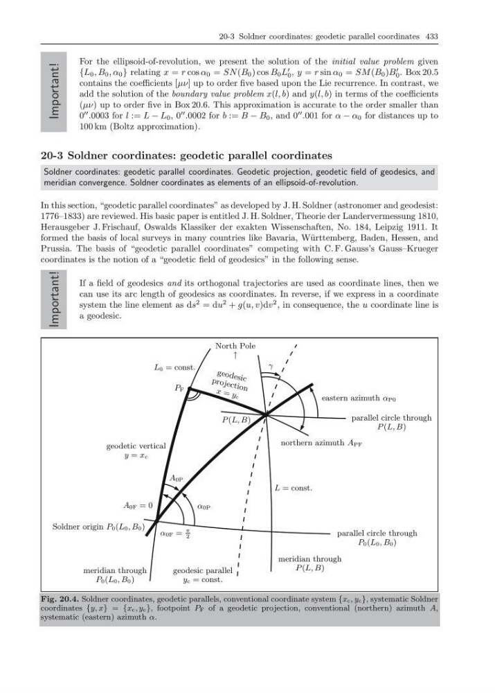
Fig. 20.4. Soldner coordinates, geodetic parallels, conventional coordinate system {x c , y c }, systematic Soldner
coordinates {y, x} = {x c , y c }, footpoint P F of a geodetic projection, conventional (northern) azimuth A,
systematic (eastern) azimuth α.
Important!
For the ellipsoid-of-revolution, we present the solution of the initial value problem given
{L 0 , B 0 , α 0 } relating x = r cos α 0 = SN (B 0 ) cos B 0 L
0 , y = r sin α 0 = SM (B 0 )B
0 . Box 20.5
contains the coefficients [µν] up to order five based upon the Lie recurrence. In contrast, we
add the solution of the boundary value problem x(l, b) and y(l, b) in terms of the coefficients
(µν) up to order five in Box 20.6. This approximation is accurate to the order smaller than
0
.0003 for l := L − L 0 , 0
.0002 for b := B − B 0 , and 0
.001 for α − α 0 for distances up to
100 km (Boltz approximation).
20-3 Soldner coordinates: geodetic parallel coordinates
Soldner coordinates: geodetic parallel coordinates. Geodetic projection, geodetic field of geodesics, and
meridian convergence. Soldner coordinates as elements of an ellipsoid-of-revolution.
In this section, “geodetic parallel coordinates” as developed by J. H. Soldner (astronomer and geodesist:
1776–1833) are reviewed. His basic paper is entitled J. H. Soldner, Theorie der Landervermessung 1810,
Herausgeber J. Frischauf, Oswalds Klassiker der exakten Wissenschaften, No. 184, Leipzig 1911. It
formed the basis of local surveys in many countries like Bavaria, W¨ urttemberg, Baden, Hessen, and
Prussia. The basis of “geodetic parallel coordinates” competing with C. F. Gauss’s Gauss–Krueger
coordinates is the notion of a “geodetic field of geodesics” in the following sense.
Important!
If a field of geodesics and its orthogonal trajectories are used as coordinate lines, then we
can use its arc length of geodesics as coordinates. In reverse, if we express in a coordinate
system the line element as ds
2 = du
2 + g(u, v)dv
2 , in consequence, the u coordinate line is
a geodesic.
Soldner origin P 0 (L 0 , B 0 )
geodesic parallel
y c = const.
g eo d es ic
p ro je ct io n
x = y c
parallel circle through
P (L, B)
parallel circle through
P 0 (L 0 , B 0 )
γ
P (L, B)
P F
L 0 = const.
L = const.
geodetic vertical
y = x c
North Pole
↑
northern azimuth A PF
eastern azimuth α P0
meridian through
P 0 (L 0 , B 0 )
α 0P
A 0P
A 0F = 0
α 0F =
π
2
meridian through
P (L, B)
Fig. 20.4. Soldner coordinates, geodetic parallels, conventional coordinate system {x c , y c }, systematic Soldner
coordinates {y, x} = {x c , y c }, footpoint P F of a geodetic projection, conventional (northern) azimuth A,
systematic (eastern) azimuth α.