

430 20 Geodetic mapping
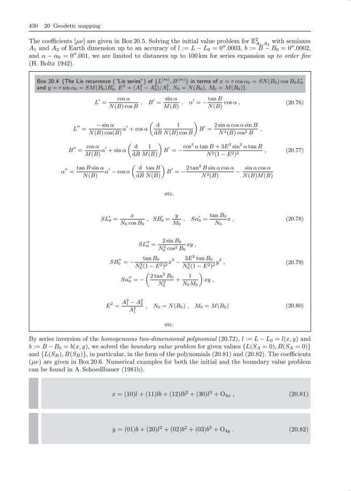
The coefficients [µν] are given in Box 20.5. Solving the initial value problem for E
2
A 1 ,A 2
with semiaxes
A 1 and A 2 of Earth dimension up to an accuracy of l := L − L 0 = 0
.0003, b := B − B 0 = 0
.0002,
and α − α 0 = 0
.001, we are limited to distances up to 100 km for series expansion up to order five
(H. Boltz 1942).
Box 20.4 (The Lie recurrence (“Lie series”) of {L
(m) , B
(m) } in terms of x = r cos α 0 = SN (B 0 ) cos B 0 L
0
and y = r sin α 0 = SM (B 0 )B
0 , E
2 = (A
2
1 − A
2
2 )/A
2
1 , N 0 = N (B 0 ), M 0 = M (B 0 )).
L
=
cos α
N (B) cos B
, B
=
sin α
M (B)
, α
= −
tan B
N (B)
cos α ,
(20.76)
L
=
− sin α
N (B) cos(B)
α
+ cos α
„
d
dB
1
N (B) cos B
«
B
=
2 sin α cos α sin B
N 2 (B) cos 2 B
,
B
=
cos α
M (B)
α
+ sin α
„
d
dB
1
M (B)
«
B
= −
cos
2 α tan B + 3E
2 sin
2 α tan B
N 2 (1 − E 2 ) 2
,
α
=
tan B sin α
N (B)
α
− cos α
„
d
dB
tan B
N (B)
«
B
= −
2 tan
2 B sin α cos α
N 2 (B)
−
sin α cos α
N (B)M (B)
(20.77)
etc.
SL
0 =
x
N 0 cos B 0
, SB
0 =
y
M 0
, Sα
0 =
tan B 0
N 0
x ,
(20.78)
SL
0 =
2 sin B 0
N
2
0 cos 2 B 0
xy ,
SB
0 = −
tan B 0
N
2
0 (1 − E 2 ) 2 x
2 −
3E
2 tan B 0
N
2
0 (1 − E 2 ) 2 y
2 ,
Sα
0 = −
„
2 tan
2 B 0
N
2
0
+
1
N 0 M 0
«
xy ,
(20.79)
E
2 =
A
2
1 − A
2
2
A
2
1
, N 0 = N (B 0 ) , M 0 = M (B 0 )
(20.80)
etc.
By series inversion of the homogeneous two-dimensional polynomial (20.72), l := L − L 0 = l(x, y) and
b := B − B 0 = b(x, y), we solved the boundary value problem for given values {L(S A = 0), B(S A = 0)}
and {L(S B ), B(S B )}, in particular, in the form of the polynomials (20.81) and (20.82). The coefficients
(µν) are given in Box 20.6. Numerical examples for both the initial and the boundary value problem
can be found in A. Schoedlbauer (1981b).
x = (10)l + (11)lb + (12)lb
2 + (30)l
3 + O 4x ,
(20.81)
y = (01)b + (20)l
2 + (02)b
2 + (03)b
3 + O 4y .
(20.82)
The coefficients [µν] are given in Box 20.5. Solving the initial value problem for E
2
A 1 ,A 2
with semiaxes
A 1 and A 2 of Earth dimension up to an accuracy of l := L − L 0 = 0
.0003, b := B − B 0 = 0
.0002,
and α − α 0 = 0
.001, we are limited to distances up to 100 km for series expansion up to order five
(H. Boltz 1942).
Box 20.4 (The Lie recurrence (“Lie series”) of {L
(m) , B
(m) } in terms of x = r cos α 0 = SN (B 0 ) cos B 0 L
0
and y = r sin α 0 = SM (B 0 )B
0 , E
2 = (A
2
1 − A
2
2 )/A
2
1 , N 0 = N (B 0 ), M 0 = M (B 0 )).
L
=
cos α
N (B) cos B
, B
=
sin α
M (B)
, α
= −
tan B
N (B)
cos α ,
(20.76)
L
=
− sin α
N (B) cos(B)
α
+ cos α
„
d
dB
1
N (B) cos B
«
B
=
2 sin α cos α sin B
N 2 (B) cos 2 B
,
B
=
cos α
M (B)
α
+ sin α
„
d
dB
1
M (B)
«
B
= −
cos
2 α tan B + 3E
2 sin
2 α tan B
N 2 (1 − E 2 ) 2
,
α
=
tan B sin α
N (B)
α
− cos α
„
d
dB
tan B
N (B)
«
B
= −
2 tan
2 B sin α cos α
N 2 (B)
−
sin α cos α
N (B)M (B)
(20.77)
etc.
SL
0 =
x
N 0 cos B 0
, SB
0 =
y
M 0
, Sα
0 =
tan B 0
N 0
x ,
(20.78)
SL
0 =
2 sin B 0
N
2
0 cos 2 B 0
xy ,
SB
0 = −
tan B 0
N
2
0 (1 − E 2 ) 2 x
2 −
3E
2 tan B 0
N
2
0 (1 − E 2 ) 2 y
2 ,
Sα
0 = −
„
2 tan
2 B 0
N
2
0
+
1
N 0 M 0
«
xy ,
(20.79)
E
2 =
A
2
1 − A
2
2
A
2
1
, N 0 = N (B 0 ) , M 0 = M (B 0 )
(20.80)
etc.
By series inversion of the homogeneous two-dimensional polynomial (20.72), l := L − L 0 = l(x, y) and
b := B − B 0 = b(x, y), we solved the boundary value problem for given values {L(S A = 0), B(S A = 0)}
and {L(S B ), B(S B )}, in particular, in the form of the polynomials (20.81) and (20.82). The coefficients
(µν) are given in Box 20.6. Numerical examples for both the initial and the boundary value problem
can be found in A. Schoedlbauer (1981b).
x = (10)l + (11)lb + (12)lb
2 + (30)l
3 + O 4x ,
(20.81)
y = (01)b + (20)l
2 + (02)b
2 + (03)b
3 + O 4y .
(20.82)