

416 20 Geodetic mapping
Section 20-1.
The elaborate presentation of Riemann polar/normal coordinates starts in Section 20-1 by the setup of
a minimal atlas of the biaxial ellipsoid, namely in terms of {ellipsoidal longitude, ellipsoidal latitude}
and {meta-longitude, meta-latitude}. Box 20.1 and Box 20.2 collect all fundamental elements of surface geometry of E
2
A 1 ,A 2
(two-dimensional ellipsoid-of-revolution, semi-major axis A 1 , semi-minor axis
A 2 ). The Darboux frame of a one-dimensional submanifold in the two-dimensional manifold E
2
A 1 ,A 2
is reviewed, in particular, by Corollary 20.3, the representation of geodetic curvature, geodetic torsion, and normal curvature in terms of elements of the first and second fundamental form as well as
of Christoffel symbols. First, we define the geodesic. Second, we define the geodesic circle following
A. Fialkow (1939), J. A. Schouten (1954), W. O. Vogel (1970, 1973) and K. Yano (1940a–d, 1942) enriched by two examples. Corollary 20.2 states that a curve is a geodesic if and only if it fulfills a system
of second order ordinary differential equations (20.42). In contrast, a curve is a geodesic circle if and
only if it fulfills a system of third order ordinary differential equations (20.43). Proofs are presented
in Appendix E-1 and E-2. Finally, we define Riemann polar/normal coordinates and by Definition 20.4
the Riemann mapping.
Section 20-2.
Section 20-2 concentrates on the computation of Riemann polar/normal coordinates. First, by solving
the two second order ordinary differential equations of a geodesic in the Lagrange portrait, namely
by means of the Legendre recurrence (“Legendre series”), in particular, initial value problem versus
boundary value problem, by the technique of standard series inversion. Second, the three first order
ordinary differential equations of a geodesic in the Hamilton portrait (“phase space”) subject to the
A. C. Clairaut constant for a rotational symmetric surface like the ellipsoid-of-revolution are solved by
means of the Lie recurrence (“Lie series”), in particular, initial value problem versus boundary value
problem, by the technique of standard series inversion.
Section 20-3.
Section 20-3 treats the elaborate Soldner coordinates or geodetic parallel coordinates. These coordinates
compete with Gauss–Krueger coordinates and Riemann normal coordinates. The way of construction
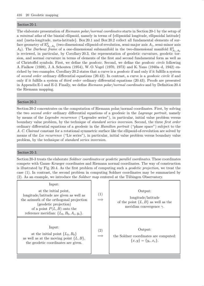
is illustrated by Fig. 20.4. As the first problem of computing such a geodetic projection, we treat the
case (1). In contrast, the second problem in computing Soldner coordinates may be summarized by
(2). As an example, we introduce the Soldner map centered at the T¨ ubingen Observatory.
=⇒
(1)
Input:
at the initial point,
longitude/latitude are given as well as
the azimuth of the orthogonal projection
(geodetic projection)
of a point P (L, B) onto the
reference meridian: {L 0 , B 0 , A c , y c }.
Output:
longitude/latitude
of the point {L, B} as well as the
meridian convergence γ.
=⇒
(2)
Input:
at the initial point {L 0 , B 0 }
as well as at the moving point {L, B},
the geodetic coordinates are given.
Output:
the Soldner coordinates are computed:
{x, y} = {y c , x c }.
Section 20-1.
The elaborate presentation of Riemann polar/normal coordinates starts in Section 20-1 by the setup of
a minimal atlas of the biaxial ellipsoid, namely in terms of {ellipsoidal longitude, ellipsoidal latitude}
and {meta-longitude, meta-latitude}. Box 20.1 and Box 20.2 collect all fundamental elements of surface geometry of E
2
A 1 ,A 2
(two-dimensional ellipsoid-of-revolution, semi-major axis A 1 , semi-minor axis
A 2 ). The Darboux frame of a one-dimensional submanifold in the two-dimensional manifold E
2
A 1 ,A 2
is reviewed, in particular, by Corollary 20.3, the representation of geodetic curvature, geodetic torsion, and normal curvature in terms of elements of the first and second fundamental form as well as
of Christoffel symbols. First, we define the geodesic. Second, we define the geodesic circle following
A. Fialkow (1939), J. A. Schouten (1954), W. O. Vogel (1970, 1973) and K. Yano (1940a–d, 1942) enriched by two examples. Corollary 20.2 states that a curve is a geodesic if and only if it fulfills a system
of second order ordinary differential equations (20.42). In contrast, a curve is a geodesic circle if and
only if it fulfills a system of third order ordinary differential equations (20.43). Proofs are presented
in Appendix E-1 and E-2. Finally, we define Riemann polar/normal coordinates and by Definition 20.4
the Riemann mapping.
Section 20-2.
Section 20-2 concentrates on the computation of Riemann polar/normal coordinates. First, by solving
the two second order ordinary differential equations of a geodesic in the Lagrange portrait, namely
by means of the Legendre recurrence (“Legendre series”), in particular, initial value problem versus
boundary value problem, by the technique of standard series inversion. Second, the three first order
ordinary differential equations of a geodesic in the Hamilton portrait (“phase space”) subject to the
A. C. Clairaut constant for a rotational symmetric surface like the ellipsoid-of-revolution are solved by
means of the Lie recurrence (“Lie series”), in particular, initial value problem versus boundary value
problem, by the technique of standard series inversion.
Section 20-3.
Section 20-3 treats the elaborate Soldner coordinates or geodetic parallel coordinates. These coordinates
compete with Gauss–Krueger coordinates and Riemann normal coordinates. The way of construction
is illustrated by Fig. 20.4. As the first problem of computing such a geodetic projection, we treat the
case (1). In contrast, the second problem in computing Soldner coordinates may be summarized by
(2). As an example, we introduce the Soldner map centered at the T¨ ubingen Observatory.
=⇒
(1)
Input:
at the initial point,
longitude/latitude are given as well as
the azimuth of the orthogonal projection
(geodetic projection)
of a point P (L, B) onto the
reference meridian: {L 0 , B 0 , A c , y c }.
Output:
longitude/latitude
of the point {L, B} as well as the
meridian convergence γ.
=⇒
(2)
Input:
at the initial point {L 0 , B 0 }
as well as at the moving point {L, B},
the geodetic coordinates are given.
Output:
the Soldner coordinates are computed:
{x, y} = {y c , x c }.