

400 18 “Sphere to cone”: pseudo-conic projections
18-22 Bonne mapping
We agree upon the postulate that the line-of-contact of the cone shall be mapped equidistantly. We
start the theory of the Bonne mapping from the following two postulates, from which follows (18.29).
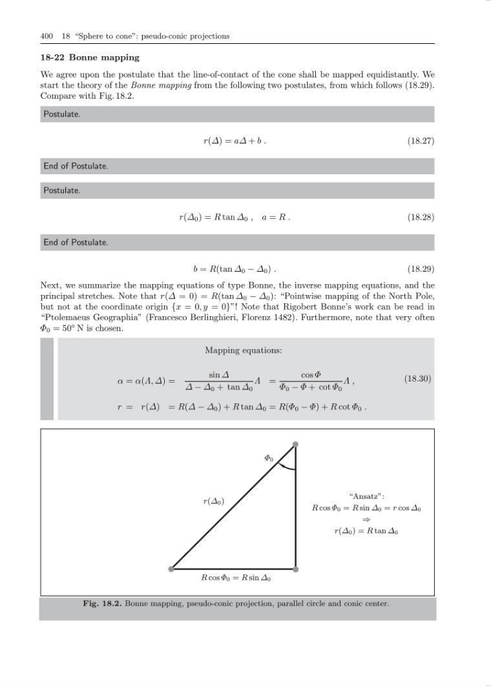
Compare with Fig. 18.2.
Postulate.
r(∆) = a∆ + b .
(18.27)
End of Postulate.
Postulate.
r(∆ 0 ) = R tan ∆ 0 , a = R .
(18.28)
End of Postulate.
b = R(tan ∆ 0 − ∆ 0 ) .
(18.29)
Next, we summarize the mapping equations of type Bonne, the inverse mapping equations, and the
principal stretches. Note that r(∆ = 0) = R(tan ∆ 0 − ∆ 0 ): “Pointwise mapping of the North Pole,
but not at the coordinate origin {x = 0, y = 0}”! Note that Rigobert Bonne’s work can be read in
“Ptolemaeus Geographia” (Francesco Berlinghieri, Florenz 1482). Furthermore, note that very often
Φ 0 = 50
◦ N is chosen.
Mapping equations:
α = α(Λ, ∆) =
sin ∆
∆ − ∆ 0 + tan ∆ 0
Λ =
cos Φ
Φ 0 − Φ + cot Φ 0
Λ ,
r = r(∆) = R(∆ − ∆ 0 ) + R tan ∆ 0 = R(Φ 0 − Φ) + R cot Φ 0 .
(18.30)
Φ 0
r(∆ 0 )
R cos Φ 0 = R sin ∆ 0
“Ansatz”:
R cos Φ 0 = R sin ∆ 0 = r cos ∆ 0
⇒
r(∆ 0 ) = R tan ∆ 0
Fig. 18.2. Bonne mapping, pseudo-conic projection, parallel circle and conic center.
18-22 Bonne mapping
We agree upon the postulate that the line-of-contact of the cone shall be mapped equidistantly. We
start the theory of the Bonne mapping from the following two postulates, from which follows (18.29).
Compare with Fig. 18.2.
Postulate.
r(∆) = a∆ + b .
(18.27)
End of Postulate.
Postulate.
r(∆ 0 ) = R tan ∆ 0 , a = R .
(18.28)
End of Postulate.
b = R(tan ∆ 0 − ∆ 0 ) .
(18.29)
Next, we summarize the mapping equations of type Bonne, the inverse mapping equations, and the
principal stretches. Note that r(∆ = 0) = R(tan ∆ 0 − ∆ 0 ): “Pointwise mapping of the North Pole,
but not at the coordinate origin {x = 0, y = 0}”! Note that Rigobert Bonne’s work can be read in
“Ptolemaeus Geographia” (Francesco Berlinghieri, Florenz 1482). Furthermore, note that very often
Φ 0 = 50
◦ N is chosen.
Mapping equations:
α = α(Λ, ∆) =
sin ∆
∆ − ∆ 0 + tan ∆ 0
Λ =
cos Φ
Φ 0 − Φ + cot Φ 0
Λ ,
r = r(∆) = R(∆ − ∆ 0 ) + R tan ∆ 0 = R(Φ 0 − Φ) + R cot Φ 0 .
(18.30)
Φ 0
r(∆ 0 )
R cos Φ 0 = R sin ∆ 0
“Ansatz”:
R cos Φ 0 = R sin ∆ 0 = r cos ∆ 0
⇒
r(∆ 0 ) = R tan ∆ 0
Fig. 18.2. Bonne mapping, pseudo-conic projection, parallel circle and conic center.