384 17 “Sphere to cone”: polar aspect
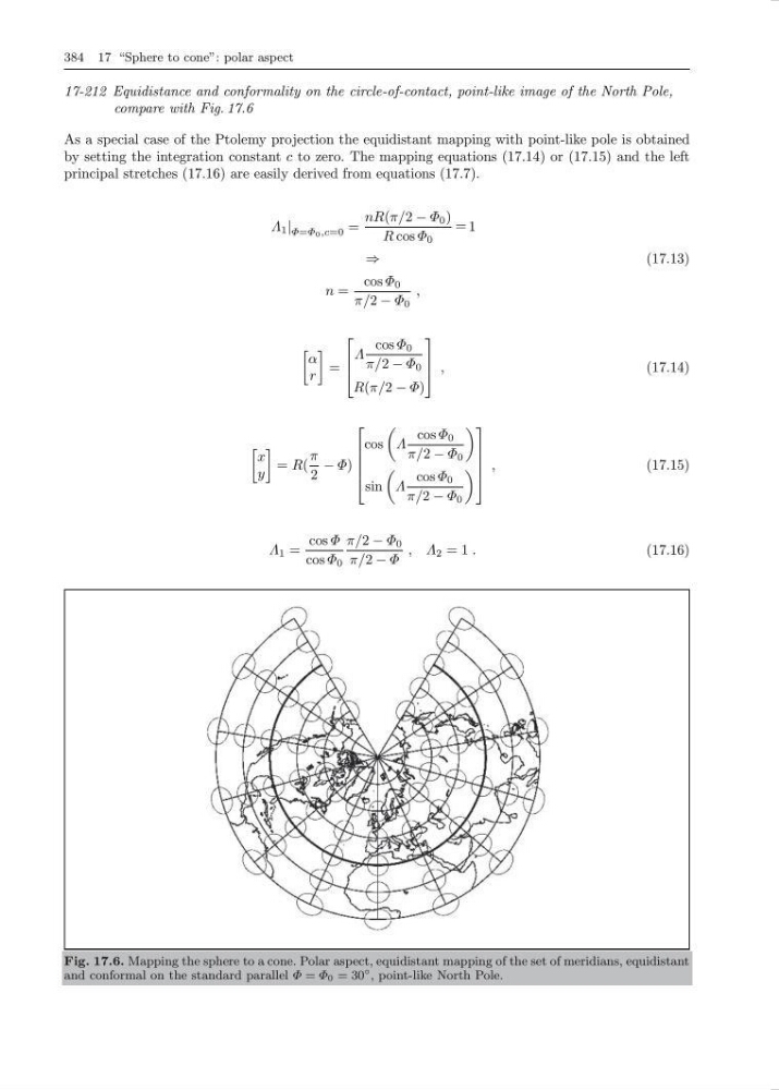
17-212 Equidistance and conformality on the circle-of-contact, point-like image of the North Pole,
compare with Fig. 17.6
As a special case of the Ptolemy projection the equidistant mapping with point-like pole is obtained
by setting the integration constant c to zero. The mapping equations (17.14) or (17.15) and the left
principal stretches (17.16) are easily derived from equations (17.7).
Λ 1 | Φ=Φ 0 ,c=0 =
nR(π/2 − Φ 0 )
R cos Φ 0
= 1
⇒
n =
cos Φ 0
π/2 − Φ 0
,
(17.13)
α
r
=
⎡
⎢
⎣
Λ
cos Φ 0
π/2 − Φ 0
R(π/2 − Φ)
⎤
⎥
⎦ ,
(17.14)
x
y
= R(
π
2
− Φ)
⎡
⎢
⎢
⎢
⎣
cos
Λ
cos Φ 0
π/2 − Φ 0
sin
Λ
cos Φ 0
π/2 − Φ 0
⎤
⎥
⎥
⎥
⎦
,
(17.15)
Λ 1 =
cos Φ
cos Φ 0
π/2 − Φ 0
π/2 − Φ
, Λ 2 = 1 .
(17.16)
Fig. 17.6. Mapping the sphere to a cone. Polar aspect, equidistant mapping of the set of meridians, equidistant
and conformal on the standard parallel Φ = Φ 0 = 30
◦ , point-like North Pole.