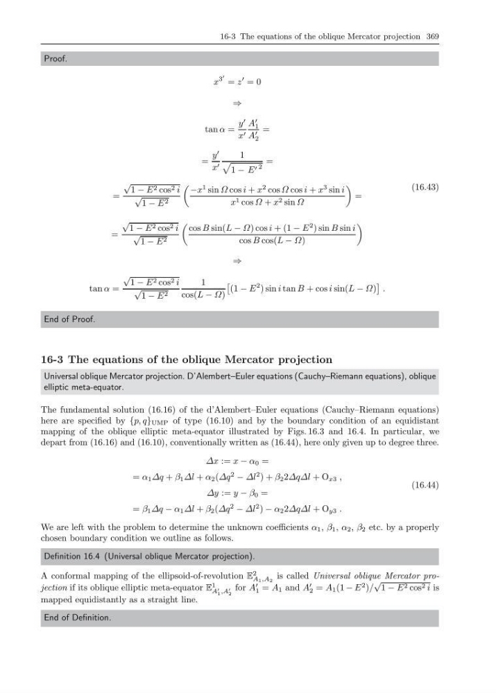
16-3 The equations of the oblique Mercator projection 369
Proof.
x
3
= z
= 0
⇒
tan α =
y
x
A
1
A
2
=
=
y
x
1
1 − E 2
=
=
√
1 − E 2 cos 2 i
√
1 − E 2
−x
1 sin Ω cos i + x
2 cos Ω cos i + x
3 sin i
x 1 cos Ω + x 2 sin Ω
=
=
√
1 − E 2 cos 2 i
√
1 − E 2
cos B sin(L − Ω) cos i + (1 − E
2 ) sin B sin i
cos B cos(L − Ω)
⇒
tan α =
√
1 − E 2 cos 2 i
√
1 − E 2
1
cos(L − Ω)
(1 − E
2 ) sin i tan B + cos i sin(L − Ω)
.
(16.43)
End of Proof.
16-3 The equations of the oblique Mercator projection
Universal oblique Mercator projection. D’Alembert–Euler equations (Cauchy–Riemann equations), oblique
elliptic meta-equator.
The fundamental solution (16.16) of the d’Alembert–Euler equations (Cauchy–Riemann equations)
here are specified by {p, q} UMP of type (16.10) and by the boundary condition of an equidistant
mapping of the oblique elliptic meta-equator illustrated by Figs. 16.3 and 16.4. In particular, we
depart from (16.16) and (16.10), conventionally written as (16.44), here only given up to degree three.
∆x := x − α 0 =
= α 1 ∆q + β 1 ∆l + α 2 (∆q
2
− ∆l
2 ) + β 2 2∆q∆l + O x3 ,
∆y := y − β 0 =
= β 1 ∆q − α 1 ∆l + β 2 (∆q
2
− ∆l
2 ) − α 2 2∆q∆l + O y3 .
(16.44)
We are left with the problem to determine the unknown coefficients α 1 , β 1 , α 2 , β 2 etc. by a properly
chosen boundary condition we outline as follows.
Definition 16.4 (Universal oblique Mercator projection).
A conformal mapping of the ellipsoid-of-revolution E
2
A 1 ,A 2
is called Universal oblique Mercator projection if its oblique elliptic meta-equator E
1
A
1 ,A
2
for A
1 = A 1 and A
2 = A 1 (1 − E
2 )/
√
1 − E 2 cos 2 i is
mapped equidistantly as a straight line.
End of Definition.