

354 15 “Ellipsoid-of-revolution to cylinder”: transverse aspect
step one
L, B
l 1 := L − L 01
b 1 := B − B 01
l 2 := L − L 02
b 2 := B − B 02
l 1 = L(x 1 , y 1 )
b 1 = B(x 1 , y 1 )
conformal polynomial inversion
step two
x 1 , y 1
x 2 , y 2
x 2 = X(x 1 , y 1 )
y 2 = Y (x 1 , y 1 )
x 2 = X lb (l 1 , b 1 ; L 01 − L 02 )
y 2 = Y lb (l 1 , b 1 ; L 01 − L 02 )
B 01 = B 02 = B 0
l 2 = (L 01 − L 02 ) + l 1
b 2 = (B 01 − B 02 ) + b 1
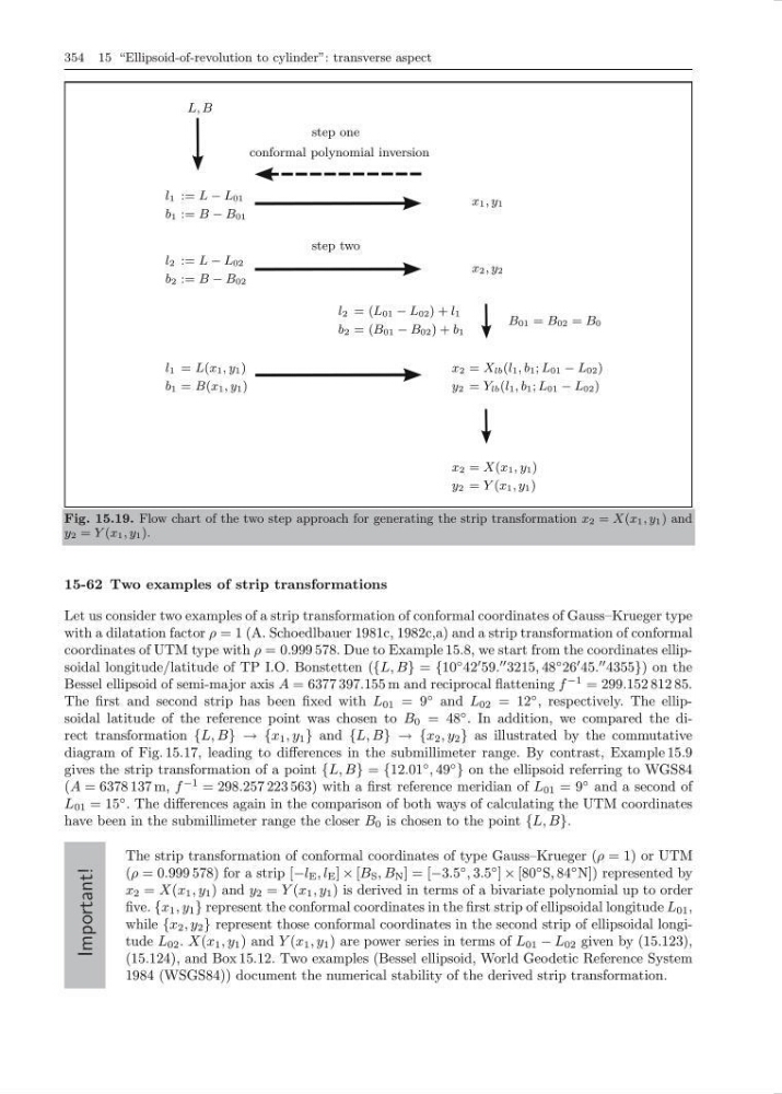
Fig. 15.19. Flow chart of the two step approach for generating the strip transformation x 2 = X(x 1 , y 1 ) and
y 2 = Y (x 1 , y 1 ).
15-62 Two examples of strip transformations
Let us consider two examples of a strip transformation of conformal coordinates of Gauss–Krueger type
with a dilatation factor ρ = 1 (A. Schoedlbauer 1981c, 1982c,a) and a strip transformation of conformal
coordinates of UTM type with ρ = 0.999 578. Due to Example 15.8, we start from the coordinates ellipsoidal longitude/latitude of TP I.O. Bonstetten ({L, B} = {10
◦ 42
59.
3215, 48
◦ 26
45.
4355}) on the
Bessel ellipsoid of semi-major axis A = 6377 397.155 m and reciprocal flattening f
−1 = 299.152 812 85.
The first and second strip has been fixed with L 01 = 9
◦ and L 02 = 12
◦ , respectively. The ellipsoidal latitude of the reference point was chosen to B 0 = 48
◦ . In addition, we compared the direct transformation {L, B} → {x 1 , y 1 } and {L, B} → {x 2 , y 2 } as illustrated by the commutative
diagram of Fig. 15.17, leading to differences in the submillimeter range. By contrast, Example 15.9
gives the strip transformation of a point {L, B} = {12.01
◦ , 49
◦
} on the ellipsoid referring to WGS84
(A = 6378 137 m, f
−1 = 298.257 223 563) with a first reference meridian of L 01 = 9
◦ and a second of
L 01 = 15
◦ . The differences again in the comparison of both ways of calculating the UTM coordinates
have been in the submillimeter range the closer B 0 is chosen to the point {L, B}.
Important!
The strip transformation of conformal coordinates of type Gauss–Krueger (ρ = 1) or UTM
(ρ = 0.999 578) for a strip [−l E , l E ] × [B S , B N ] = [−3.5
◦ , 3.5
◦ ] × [80
◦ S, 84
◦ N]) represented by
x 2 = X(x 1 , y 1 ) and y 2 = Y (x 1 , y 1 ) is derived in terms of a bivariate polynomial up to order
five. {x 1 , y 1 } represent the conformal coordinates in the first strip of ellipsoidal longitude L 01 ,
while {x 2 , y 2 } represent those conformal coordinates in the second strip of ellipsoidal longitude L 02 . X(x 1 , y 1 ) and Y (x 1 , y 1 ) are power series in terms of L 01 − L 02 given by (15.123),
(15.124), and Box 15.12. Two examples (Bessel ellipsoid, World Geodetic Reference System
1984 (WSGS84)) document the numerical stability of the derived strip transformation.
step one
L, B
l 1 := L − L 01
b 1 := B − B 01
l 2 := L − L 02
b 2 := B − B 02
l 1 = L(x 1 , y 1 )
b 1 = B(x 1 , y 1 )
conformal polynomial inversion
step two
x 1 , y 1
x 2 , y 2
x 2 = X(x 1 , y 1 )
y 2 = Y (x 1 , y 1 )
x 2 = X lb (l 1 , b 1 ; L 01 − L 02 )
y 2 = Y lb (l 1 , b 1 ; L 01 − L 02 )
B 01 = B 02 = B 0
l 2 = (L 01 − L 02 ) + l 1
b 2 = (B 01 − B 02 ) + b 1
Fig. 15.19. Flow chart of the two step approach for generating the strip transformation x 2 = X(x 1 , y 1 ) and
y 2 = Y (x 1 , y 1 ).
15-62 Two examples of strip transformations
Let us consider two examples of a strip transformation of conformal coordinates of Gauss–Krueger type
with a dilatation factor ρ = 1 (A. Schoedlbauer 1981c, 1982c,a) and a strip transformation of conformal
coordinates of UTM type with ρ = 0.999 578. Due to Example 15.8, we start from the coordinates ellipsoidal longitude/latitude of TP I.O. Bonstetten ({L, B} = {10
◦ 42
59.
3215, 48
◦ 26
45.
4355}) on the
Bessel ellipsoid of semi-major axis A = 6377 397.155 m and reciprocal flattening f
−1 = 299.152 812 85.
The first and second strip has been fixed with L 01 = 9
◦ and L 02 = 12
◦ , respectively. The ellipsoidal latitude of the reference point was chosen to B 0 = 48
◦ . In addition, we compared the direct transformation {L, B} → {x 1 , y 1 } and {L, B} → {x 2 , y 2 } as illustrated by the commutative
diagram of Fig. 15.17, leading to differences in the submillimeter range. By contrast, Example 15.9
gives the strip transformation of a point {L, B} = {12.01
◦ , 49
◦
} on the ellipsoid referring to WGS84
(A = 6378 137 m, f
−1 = 298.257 223 563) with a first reference meridian of L 01 = 9
◦ and a second of
L 01 = 15
◦ . The differences again in the comparison of both ways of calculating the UTM coordinates
have been in the submillimeter range the closer B 0 is chosen to the point {L, B}.
Important!
The strip transformation of conformal coordinates of type Gauss–Krueger (ρ = 1) or UTM
(ρ = 0.999 578) for a strip [−l E , l E ] × [B S , B N ] = [−3.5
◦ , 3.5
◦ ] × [80
◦ S, 84
◦ N]) represented by
x 2 = X(x 1 , y 1 ) and y 2 = Y (x 1 , y 1 ) is derived in terms of a bivariate polynomial up to order
five. {x 1 , y 1 } represent the conformal coordinates in the first strip of ellipsoidal longitude L 01 ,
while {x 2 , y 2 } represent those conformal coordinates in the second strip of ellipsoidal longitude L 02 . X(x 1 , y 1 ) and Y (x 1 , y 1 ) are power series in terms of L 01 − L 02 given by (15.123),
(15.124), and Box 15.12. Two examples (Bessel ellipsoid, World Geodetic Reference System
1984 (WSGS84)) document the numerical stability of the derived strip transformation.