

15-6 Strip transformation of conformal coordinates (Gauss–Krueger/UTM mappings) 347
15-61 Two-step-approach to strip transformations
Here, we outline the two-step-approach which leads us by inversion technology of bivariate homogeneous polynomials to the strip transformation x 2 = X(x 1 , y 1 ) and y 2 = Y (x 1 , y 1 ) of conformal
coordinates {x 1 , y 1 } of the first L 01 -strip into conformal coordinates {x 2 , y 2 } of the second L 02 -strip,
namely for conformal coordinates of type Gauss–Krueger (GK) and UTM.
x 2 = X(x 1 , y 1 )
y 2 = X(x 1 , y 1 )
{x 1 , y 1 }
GK or UTM
L 01
{x 2 , y 2 }
GK or UTM
L 02
x 1 = f 1 (L, B)
y 1 = g 1 (L, B)
x 2 = f 2 (L, B)
y 2 = g 2 (L, B)
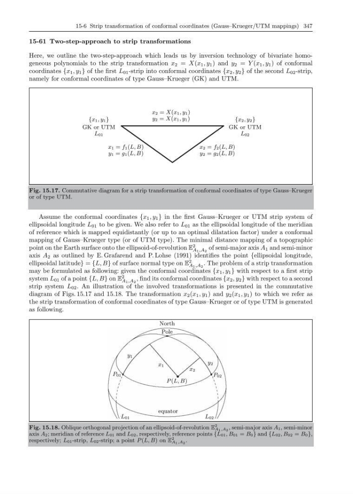
Fig. 15.17. Commutative diagram for a strip transformation of conformal coordinates of type Gauss–Krueger
or of type UTM.
Assume the conformal coordinates {x 1 , y 1 } in the first Gauss–Krueger or UTM strip system of
ellipsoidal longitude L 01 to be given. We also refer to L 01 as the ellipsoidal longitude of the meridian
of reference which is mapped equidistantly (or up to an optimal dilatation factor) under a conformal
mapping of Gauss–Krueger type (or of UTM type). The minimal distance mapping of a topographic
point on the Earth surface onto the ellipsoid-of-revolution E
2
A 1 ,A 2
of semi-major axis A 1 and semi-minor
axis A 2 as outlined by E. Grafarend and P. Lohse (1991) identifies the point {ellipsoidal longitude,
ellipsoidal latitude} = {L, B} of surface normal type on E
2
A 1 ,A 2
. The problem of a strip transformation
may be formulated as following: given the conformal coordinates {x 1 , y 1 } with respect to a first strip
system L 01 of a point {L, B} on E
2
A 1 ,A 2
, find its conformal coordinates {x 2 , y 2 } with respect to a second
strip system L 02 . An illustration of the involved transformations is presented in the commutative
diagram of Figs. 15.17 and 15.18. The transformation x 2 (x 1 , y 1 ) and y 2 (x 1 , y 1 ) to which we refer as
the strip transformation of conformal coordinates of type Gauss–Krueger or of type UTM is generated
as following.
equator
North
Pole
P (L, B)
y 2
x 1
x 2
y 1
P 01
P 02
L 01
L 02
Fig. 15.18. Oblique orthogonal projection of an ellipsoid-of-revolution E
2
A 1 ,A 2 , semi-major axis A 1 , semi-minor
axis A 2 ; meridian of reference L 01 and L 02 , respectively, reference points {L 01 , B 01 = B 0 } and {L 02 , B 02 = B 0 },
respectively; L 01 -strip, L 02 -strip; a point P (L, B) on E
2
A 1 ,A 2 .
15-61 Two-step-approach to strip transformations
Here, we outline the two-step-approach which leads us by inversion technology of bivariate homogeneous polynomials to the strip transformation x 2 = X(x 1 , y 1 ) and y 2 = Y (x 1 , y 1 ) of conformal
coordinates {x 1 , y 1 } of the first L 01 -strip into conformal coordinates {x 2 , y 2 } of the second L 02 -strip,
namely for conformal coordinates of type Gauss–Krueger (GK) and UTM.
x 2 = X(x 1 , y 1 )
y 2 = X(x 1 , y 1 )
{x 1 , y 1 }
GK or UTM
L 01
{x 2 , y 2 }
GK or UTM
L 02
x 1 = f 1 (L, B)
y 1 = g 1 (L, B)
x 2 = f 2 (L, B)
y 2 = g 2 (L, B)
Fig. 15.17. Commutative diagram for a strip transformation of conformal coordinates of type Gauss–Krueger
or of type UTM.
Assume the conformal coordinates {x 1 , y 1 } in the first Gauss–Krueger or UTM strip system of
ellipsoidal longitude L 01 to be given. We also refer to L 01 as the ellipsoidal longitude of the meridian
of reference which is mapped equidistantly (or up to an optimal dilatation factor) under a conformal
mapping of Gauss–Krueger type (or of UTM type). The minimal distance mapping of a topographic
point on the Earth surface onto the ellipsoid-of-revolution E
2
A 1 ,A 2
of semi-major axis A 1 and semi-minor
axis A 2 as outlined by E. Grafarend and P. Lohse (1991) identifies the point {ellipsoidal longitude,
ellipsoidal latitude} = {L, B} of surface normal type on E
2
A 1 ,A 2
. The problem of a strip transformation
may be formulated as following: given the conformal coordinates {x 1 , y 1 } with respect to a first strip
system L 01 of a point {L, B} on E
2
A 1 ,A 2
, find its conformal coordinates {x 2 , y 2 } with respect to a second
strip system L 02 . An illustration of the involved transformations is presented in the commutative
diagram of Figs. 15.17 and 15.18. The transformation x 2 (x 1 , y 1 ) and y 2 (x 1 , y 1 ) to which we refer as
the strip transformation of conformal coordinates of type Gauss–Krueger or of type UTM is generated
as following.
equator
North
Pole
P (L, B)
y 2
x 1
x 2
y 1
P 01
P 02
L 01
L 02
Fig. 15.18. Oblique orthogonal projection of an ellipsoid-of-revolution E
2
A 1 ,A 2 , semi-major axis A 1 , semi-minor
axis A 2 ; meridian of reference L 01 and L 02 , respectively, reference points {L 01 , B 01 = B 0 } and {L 02 , B 02 = B 0 },
respectively; L 01 -strip, L 02 -strip; a point P (L, B) on E
2
A 1 ,A 2 .