

332 15 “Ellipsoid-of-revolution to cylinder”: transverse aspect
Example 15.3 ([−l E , +l E ] × [B S , B N ] = [−3.5
◦ , +3.5
◦ ] × [80
◦ S, 84
◦ N]).
The classical UTM conformal coordinate system is chosen for a strip of 6
◦ width with 1
◦ overlays and
between B S = −80
◦ of southern latitude and B N = +84
◦ of northern latitude. Once we refer to the
Geodetic Reference System 1980 (H. Moritz, 1984), E
2 = 0.006 694 380 022 90, in particular, with l E
given by l E = 3.5
◦ = 0.061 086 5 rad, the dilatation parameter amounts to
ρ = 0.999 578 (scale reduction factor 1 : 2 370) .
(15.101)
End of Example.
Example 15.4 ([−l E , +l E ] × [B S , B N ] = [−2
◦ , +2
◦ ] × [80
◦ S, 80
◦ N]).
The classical Gauss–Krueger conformal coordinate system is chosen for a strip of 3
◦ width with 0.5
◦
overlays and between B S = −80
◦ of southern latitude and B N = +80
◦ of northern latitude. Once we
refer to the Geodetic Reference System 1980, E
2 = 0.006 694 380 022 90, in particular, with l E given
by l E = 2
◦ = 0.034 906 5 rad, the dilatation parameter amounts to
ρ = 0.999 864 (scale reduction factor 1 : 7 353) .
(15.102)
End of Example.
1 − ρ
0.000420
0.000419
0.000418
0.000417
0.000416
0.000415
10
−4 10
−3 10
−2 10
−1 1 E
(5)
1 − ρ
0.0004
0.0002
0
0
◦
1
◦
2
◦
3
◦
l E
(3)
(4)
1 − ρ
0.0006
0.0005
0
1 /2
1 E
Λ/ρ − 1
l
0
0.0001
0.0002
0
◦
1
◦
2
◦
3
◦
(1)
(2)
Λ/ρ − 1
B
0
0.0004
0.0008
0.0012
0
◦
20
◦
40
◦
60
◦
80
◦
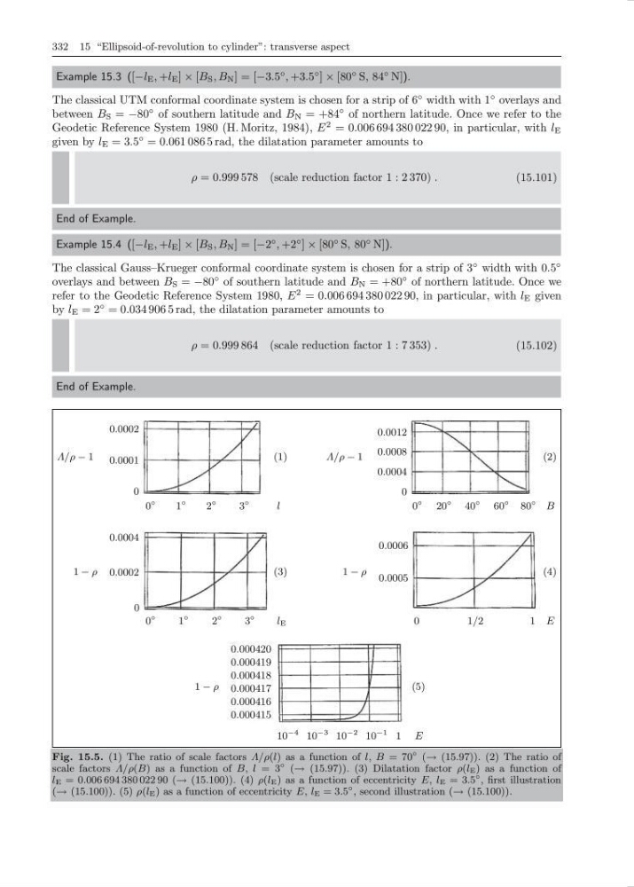
Fig. 15.5. (1) The ratio of scale factors Λ/ρ(l) as a function of l, B = 70
◦ (→ (15.97)). (2) The ratio of
scale factors Λ/ρ(B) as a function of B, l = 3
◦ (→ (15.97)). (3) Dilatation factor ρ(l E ) as a function of
l E = 0.006 694 380 022 90 (→ (15.100)). (4) ρ(l E ) as a function of eccentricity E, l E = 3.5
◦ , first illustration
(→ (15.100)). (5) ρ(l E ) as a function of eccentricity E, l E = 3.5
◦ , second illustration (→ (15.100)).
Example 15.3 ([−l E , +l E ] × [B S , B N ] = [−3.5
◦ , +3.5
◦ ] × [80
◦ S, 84
◦ N]).
The classical UTM conformal coordinate system is chosen for a strip of 6
◦ width with 1
◦ overlays and
between B S = −80
◦ of southern latitude and B N = +84
◦ of northern latitude. Once we refer to the
Geodetic Reference System 1980 (H. Moritz, 1984), E
2 = 0.006 694 380 022 90, in particular, with l E
given by l E = 3.5
◦ = 0.061 086 5 rad, the dilatation parameter amounts to
ρ = 0.999 578 (scale reduction factor 1 : 2 370) .
(15.101)
End of Example.
Example 15.4 ([−l E , +l E ] × [B S , B N ] = [−2
◦ , +2
◦ ] × [80
◦ S, 80
◦ N]).
The classical Gauss–Krueger conformal coordinate system is chosen for a strip of 3
◦ width with 0.5
◦
overlays and between B S = −80
◦ of southern latitude and B N = +80
◦ of northern latitude. Once we
refer to the Geodetic Reference System 1980, E
2 = 0.006 694 380 022 90, in particular, with l E given
by l E = 2
◦ = 0.034 906 5 rad, the dilatation parameter amounts to
ρ = 0.999 864 (scale reduction factor 1 : 7 353) .
(15.102)
End of Example.
1 − ρ
0.000420
0.000419
0.000418
0.000417
0.000416
0.000415
10
−4 10
−3 10
−2 10
−1 1 E
(5)
1 − ρ
0.0004
0.0002
0
0
◦
1
◦
2
◦
3
◦
l E
(3)
(4)
1 − ρ
0.0006
0.0005
0
1 /2
1 E
Λ/ρ − 1
l
0
0.0001
0.0002
0
◦
1
◦
2
◦
3
◦
(1)
(2)
Λ/ρ − 1
B
0
0.0004
0.0008
0.0012
0
◦
20
◦
40
◦
60
◦
80
◦
Fig. 15.5. (1) The ratio of scale factors Λ/ρ(l) as a function of l, B = 70
◦ (→ (15.97)). (2) The ratio of
scale factors Λ/ρ(B) as a function of B, l = 3
◦ (→ (15.97)). (3) Dilatation factor ρ(l E ) as a function of
l E = 0.006 694 380 022 90 (→ (15.100)). (4) ρ(l E ) as a function of eccentricity E, l E = 3.5
◦ , first illustration
(→ (15.100)). (5) ρ(l E ) as a function of eccentricity E, l E = 3.5
◦ , second illustration (→ (15.100)).