

326 15 “Ellipsoid-of-revolution to cylinder”: transverse aspect
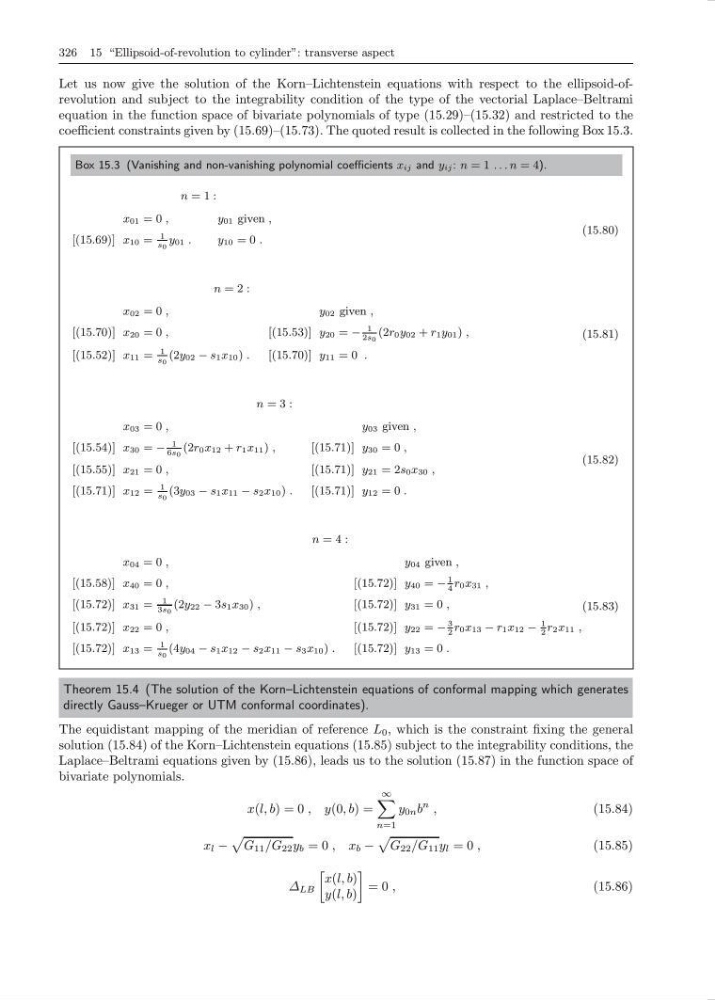
Let us now give the solution of the Korn–Lichtenstein equations with respect to the ellipsoid-ofrevolution and subject to the integrability condition of the type of the vectorial Laplace–Beltrami
equation in the function space of bivariate polynomials of type (15.29)–(15.32) and restricted to the
coefficient constraints given by (15.69)–(15.73). The quoted result is collected in the following Box 15.3.
Box 15.3 (Vanishing and non-vanishing polynomial coefficients x ij and y ij : n = 1 . . . n = 4).
n = 1 :
x 01 = 0 ,
y 01 given ,
[(15.69)] x 10 =
1
s 0
y 01 .
y 10 = 0 .
(15.80)
n = 2 :
x 02 = 0 ,
y 02 given ,
[(15.70)] x 20 = 0 ,
[(15.53)] y 20 = −
1
2s 0
(2r 0 y 02 + r 1 y 01 ) ,
[(15.52)] x 11 =
1
s 0
(2y 02 − s 1 x 10 ) .
[(15.70)] y 11 = 0 .
(15.81)
n = 3 :
x 03 = 0 ,
y 03 given ,
[(15.54)] x 30 = −
1
6s 0
(2r 0 x 12 + r 1 x 11 ) ,
[(15.71)] y 30 = 0 ,
[(15.55)] x 21 = 0 ,
[(15.71)] y 21 = 2s 0 x 30 ,
[(15.71)] x 12 =
1
s 0
(3y 03 − s 1 x 11 − s 2 x 10 ) .
[(15.71)] y 12 = 0 .
(15.82)
n = 4 :
x 04 = 0 ,
y 04 given ,
[(15.58)] x 40 = 0 ,
[(15.72)] y 40 = −
1
4
r 0 x 31 ,
[(15.72)] x 31 =
1
3s 0
(2y 22 − 3s 1 x 30 ) ,
[(15.72)] y 31 = 0 ,
[(15.72)] x 22 = 0 ,
[(15.72)] y 22 = −
3
2
r 0 x 13 − r 1 x 12 −
1
2
r 2 x 11 ,
[(15.72)] x 13 =
1
s 0
(4y 04 − s 1 x 12 − s 2 x 11 − s 3 x 10 ) .
[(15.72)] y 13 = 0 .
(15.83)
Theorem 15.4 (The solution of the Korn–Lichtenstein equations of conformal mapping which generates
directly Gauss–Krueger or UTM conformal coordinates).
The equidistant mapping of the meridian of reference L 0 , which is the constraint fixing the general
solution (15.84) of the Korn–Lichtenstein equations (15.85) subject to the integrability conditions, the
Laplace–Beltrami equations given by (15.86), leads us to the solution (15.87) in the function space of
bivariate polynomials.
x(l, b) = 0 , y(0, b) =
∞
n=1
y 0n b
n ,
(15.84)
x l −
G 11 /G 22 y b = 0 , x b −
G 22 /G 11 y l = 0 ,
(15.85)
∆ LB
x(l, b)
y(l, b)
= 0 ,
(15.86)
Let us now give the solution of the Korn–Lichtenstein equations with respect to the ellipsoid-ofrevolution and subject to the integrability condition of the type of the vectorial Laplace–Beltrami
equation in the function space of bivariate polynomials of type (15.29)–(15.32) and restricted to the
coefficient constraints given by (15.69)–(15.73). The quoted result is collected in the following Box 15.3.
Box 15.3 (Vanishing and non-vanishing polynomial coefficients x ij and y ij : n = 1 . . . n = 4).
n = 1 :
x 01 = 0 ,
y 01 given ,
[(15.69)] x 10 =
1
s 0
y 01 .
y 10 = 0 .
(15.80)
n = 2 :
x 02 = 0 ,
y 02 given ,
[(15.70)] x 20 = 0 ,
[(15.53)] y 20 = −
1
2s 0
(2r 0 y 02 + r 1 y 01 ) ,
[(15.52)] x 11 =
1
s 0
(2y 02 − s 1 x 10 ) .
[(15.70)] y 11 = 0 .
(15.81)
n = 3 :
x 03 = 0 ,
y 03 given ,
[(15.54)] x 30 = −
1
6s 0
(2r 0 x 12 + r 1 x 11 ) ,
[(15.71)] y 30 = 0 ,
[(15.55)] x 21 = 0 ,
[(15.71)] y 21 = 2s 0 x 30 ,
[(15.71)] x 12 =
1
s 0
(3y 03 − s 1 x 11 − s 2 x 10 ) .
[(15.71)] y 12 = 0 .
(15.82)
n = 4 :
x 04 = 0 ,
y 04 given ,
[(15.58)] x 40 = 0 ,
[(15.72)] y 40 = −
1
4
r 0 x 31 ,
[(15.72)] x 31 =
1
3s 0
(2y 22 − 3s 1 x 30 ) ,
[(15.72)] y 31 = 0 ,
[(15.72)] x 22 = 0 ,
[(15.72)] y 22 = −
3
2
r 0 x 13 − r 1 x 12 −
1
2
r 2 x 11 ,
[(15.72)] x 13 =
1
s 0
(4y 04 − s 1 x 12 − s 2 x 11 − s 3 x 10 ) .
[(15.72)] y 13 = 0 .
(15.83)
Theorem 15.4 (The solution of the Korn–Lichtenstein equations of conformal mapping which generates
directly Gauss–Krueger or UTM conformal coordinates).
The equidistant mapping of the meridian of reference L 0 , which is the constraint fixing the general
solution (15.84) of the Korn–Lichtenstein equations (15.85) subject to the integrability conditions, the
Laplace–Beltrami equations given by (15.86), leads us to the solution (15.87) in the function space of
bivariate polynomials.
x(l, b) = 0 , y(0, b) =
∞
n=1
y 0n b
n ,
(15.84)
x l −
G 11 /G 22 y b = 0 , x b −
G 22 /G 11 y l = 0 ,
(15.85)
∆ LB
x(l, b)
y(l, b)
= 0 ,
(15.86)