

6 “Sphere to tangential plane”: transverse aspect
Mapping the sphere to a tangential plane: meta-azimuthal projections in the transverse aspect. Equidistant, conformal (stereographic), and equal area (transverse Lambert) mappings.
Azimuthal projections may be classified by reference to the point-of-contact of the plotting surface with
the Earth. While chapter 5 treated the case of a polar azimuthal projections (azimuthal projection
in the polar aspect), this section concentrates on meta-azimuthal mappings of the Earth onto a
plane in the transverse aspect, which are often also called equatorial: the point-of-contact (metaNorth Pole) may be any point on the (conventional) equator of the reference sphere. According to
chapter 3, its spherical coordinates, referring to the equatorial frame of reference, are specified through
Λ 0 ∈ [0
◦ , 360
◦ ], Φ 0 = 0
◦ . In the special case Λ 0 = 270
◦ , the meta-North Pole is located in the West
Pole and the meta-equator (then called transverse equator) agrees with the Greenwich meridian of
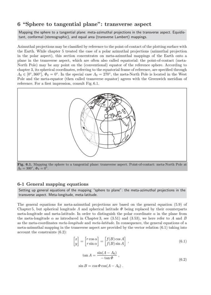
reference. For a first impression, consult Fig. 6.1.
Fig. 6.1. Mapping the sphere to a tangential plane: transverse aspect. Point-of-contact: meta-North Pole at
Λ 0 = 300
◦ , Φ 0 = 0
◦ .
6-1 General mapping equations
Setting up general equations of the mapping “sphere to plane”: the meta-azimuthal projections in the
transverse aspect. Meta-longitude, meta-latitude.
The general equations for meta-azimuthal projections are based on the general equation (5.9) of
Chapter 5, but spherical longitude Λ and spherical latitude Φ being replaced by their counterparts
meta-longitude and meta-latitude. In order to distinguish the polar coordinate α in the plane from
the meta-longitude α as introduced in Chapter 3, see (3.51) and (3.53), we here refer to A and B
as the meta-coordinates meta-longitude and meta-latitude. In consequence, the general equations of a
meta-azimuthal mapping in the transverse aspect are provided by the vector relation (6.1) taking into
account the constraints (6.2):
x
y
=
r cos α
r sin α
=
f (B) cos A
f (B) sin A
,
(6.1)
tan A =
sin(Λ − Λ 0 )
− tan Φ
,
sin B = cos Φ cos(Λ − Λ 0 ) .
(6.2)
Mapping the sphere to a tangential plane: meta-azimuthal projections in the transverse aspect. Equidistant, conformal (stereographic), and equal area (transverse Lambert) mappings.
Azimuthal projections may be classified by reference to the point-of-contact of the plotting surface with
the Earth. While chapter 5 treated the case of a polar azimuthal projections (azimuthal projection
in the polar aspect), this section concentrates on meta-azimuthal mappings of the Earth onto a
plane in the transverse aspect, which are often also called equatorial: the point-of-contact (metaNorth Pole) may be any point on the (conventional) equator of the reference sphere. According to
chapter 3, its spherical coordinates, referring to the equatorial frame of reference, are specified through
Λ 0 ∈ [0
◦ , 360
◦ ], Φ 0 = 0
◦ . In the special case Λ 0 = 270
◦ , the meta-North Pole is located in the West
Pole and the meta-equator (then called transverse equator) agrees with the Greenwich meridian of
reference. For a first impression, consult Fig. 6.1.
Fig. 6.1. Mapping the sphere to a tangential plane: transverse aspect. Point-of-contact: meta-North Pole at
Λ 0 = 300
◦ , Φ 0 = 0
◦ .
6-1 General mapping equations
Setting up general equations of the mapping “sphere to plane”: the meta-azimuthal projections in the
transverse aspect. Meta-longitude, meta-latitude.
The general equations for meta-azimuthal projections are based on the general equation (5.9) of
Chapter 5, but spherical longitude Λ and spherical latitude Φ being replaced by their counterparts
meta-longitude and meta-latitude. In order to distinguish the polar coordinate α in the plane from
the meta-longitude α as introduced in Chapter 3, see (3.51) and (3.53), we here refer to A and B
as the meta-coordinates meta-longitude and meta-latitude. In consequence, the general equations of a
meta-azimuthal mapping in the transverse aspect are provided by the vector relation (6.1) taking into
account the constraints (6.2):
x
y
=
r cos α
r sin α
=
f (B) cos A
f (B) sin A
,
(6.1)
tan A =
sin(Λ − Λ 0 )
− tan Φ
,
sin B = cos Φ cos(Λ − Λ 0 ) .
(6.2)