

5-3 The pseudo-azimuthal projection 203
category A
category B
category C
category D
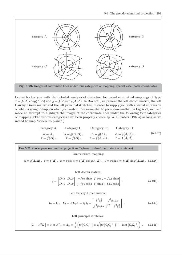
Fig. 5.29. Images of coordinate lines under four categories of mapping, special case: polar coordinates.
Let us bother you with the detailed analysis of distortion for pseudo-azimuthal mappings of type
x = f (∆) cos g(Λ, ∆) and y = f (∆) sin g(Λ, ∆). In Box 5.21, we present the left Jacobi matrix, the left
Cauchy–Green matrix and the left principal stretches. In order to supply you with a visual impression
of what is going to happen when you switch from azimuthal to pseudo-azimuthal, in Fig. 5.29, we have
made an attempt to highlight the images of the coordinate lines under the following four categories
of mapping. (The various categories have been properly chosen by W. R. Tobler (1963a) as long as we
intend to map “sphere to plane”.)
Category A:
Category B:
Category C:
Category D:
α = Λ ,
r = f (∆) .
α = g(Λ, ∆) ,
r = f (∆) .
α = g(Λ) ,
r = f (Λ, ∆) .
α = g(Λ, ∆) ,
r = f (Λ, ∆) .
(5.137)
Box 5.21 (Polar pseudo-azimuthal projections “sphere to plane”, left principal stretches).
Parameterized mapping:
α = g(Λ, ∆) , r = f (∆) , x = r cos α = f (∆) cos g(Λ, ∆) , y = r sin α = f (∆) sin g(Λ, ∆) . (5.138)
Left Jacobi matrix:
J l =
"
D Λ x D ∆ x
D Λ y D ∆ y
# " −fg Λ sin g f
cos g − fg ∆ sin g
+fg Λ cos g f
sin g + fg ∆ cos g
#
.
(5.139)
Left Cauchy–Green matrix:
G r = I 2 , C l = J
∗
l G r J l = J
∗
l J l =
"
f
2 g
2
Λ
f
2 g Λ g ∆
f
2 g Λ g ∆ f
2 + f
2 g
2
∆
#
.
(5.140)
Left principal stretches:
˛
˛ C l − Λ
2 G l
˛
˛ = 0 ⇔ Λ
2
1,2 = Λ
2
± =
1
2
„
tr
ˆ
C l G
−1
l
˜ ±
q `
tr
ˆ
C l G
−1
l
˜´ 2 − 4det
ˆ
C l G
−1
l
˜
«
,
(5.141)
category A
category B
category C
category D
Fig. 5.29. Images of coordinate lines under four categories of mapping, special case: polar coordinates.
Let us bother you with the detailed analysis of distortion for pseudo-azimuthal mappings of type
x = f (∆) cos g(Λ, ∆) and y = f (∆) sin g(Λ, ∆). In Box 5.21, we present the left Jacobi matrix, the left
Cauchy–Green matrix and the left principal stretches. In order to supply you with a visual impression
of what is going to happen when you switch from azimuthal to pseudo-azimuthal, in Fig. 5.29, we have
made an attempt to highlight the images of the coordinate lines under the following four categories
of mapping. (The various categories have been properly chosen by W. R. Tobler (1963a) as long as we
intend to map “sphere to plane”.)
Category A:
Category B:
Category C:
Category D:
α = Λ ,
r = f (∆) .
α = g(Λ, ∆) ,
r = f (∆) .
α = g(Λ) ,
r = f (Λ, ∆) .
α = g(Λ, ∆) ,
r = f (Λ, ∆) .
(5.137)
Box 5.21 (Polar pseudo-azimuthal projections “sphere to plane”, left principal stretches).
Parameterized mapping:
α = g(Λ, ∆) , r = f (∆) , x = r cos α = f (∆) cos g(Λ, ∆) , y = r sin α = f (∆) sin g(Λ, ∆) . (5.138)
Left Jacobi matrix:
J l =
"
D Λ x D ∆ x
D Λ y D ∆ y
# " −fg Λ sin g f
cos g − fg ∆ sin g
+fg Λ cos g f
sin g + fg ∆ cos g
#
.
(5.139)
Left Cauchy–Green matrix:
G r = I 2 , C l = J
∗
l G r J l = J
∗
l J l =
"
f
2 g
2
Λ
f
2 g Λ g ∆
f
2 g Λ g ∆ f
2 + f
2 g
2
∆
#
.
(5.140)
Left principal stretches:
˛
˛ C l − Λ
2 G l
˛
˛ = 0 ⇔ Λ
2
1,2 = Λ
2
± =
1
2
„
tr
ˆ
C l G
−1
l
˜ ±
q `
tr
ˆ
C l G
−1
l
˜´ 2 − 4det
ˆ
C l G
−1
l
˜
«
,
(5.141)