

5-2 Special mapping equations 197
5-25 What are the best polar azimuthal projections of “sphere to plane”?
Most textbooks on map projections list those many azimuthal projections of the “sphere to plane”
without taking any decision of which one may be the best. Indeed, for such a decision, we need an
objective criterion, and we choose it according to Chapter 1 and Chapter 2, i. e. we choose the distortion
energy over a spherical cap being covered by the chosen azimuthal projection of the sphere S
2
R to the
tangent space T N S
2
R or the plane P
2
O . In order to prepare us for a rational decision of the best polar
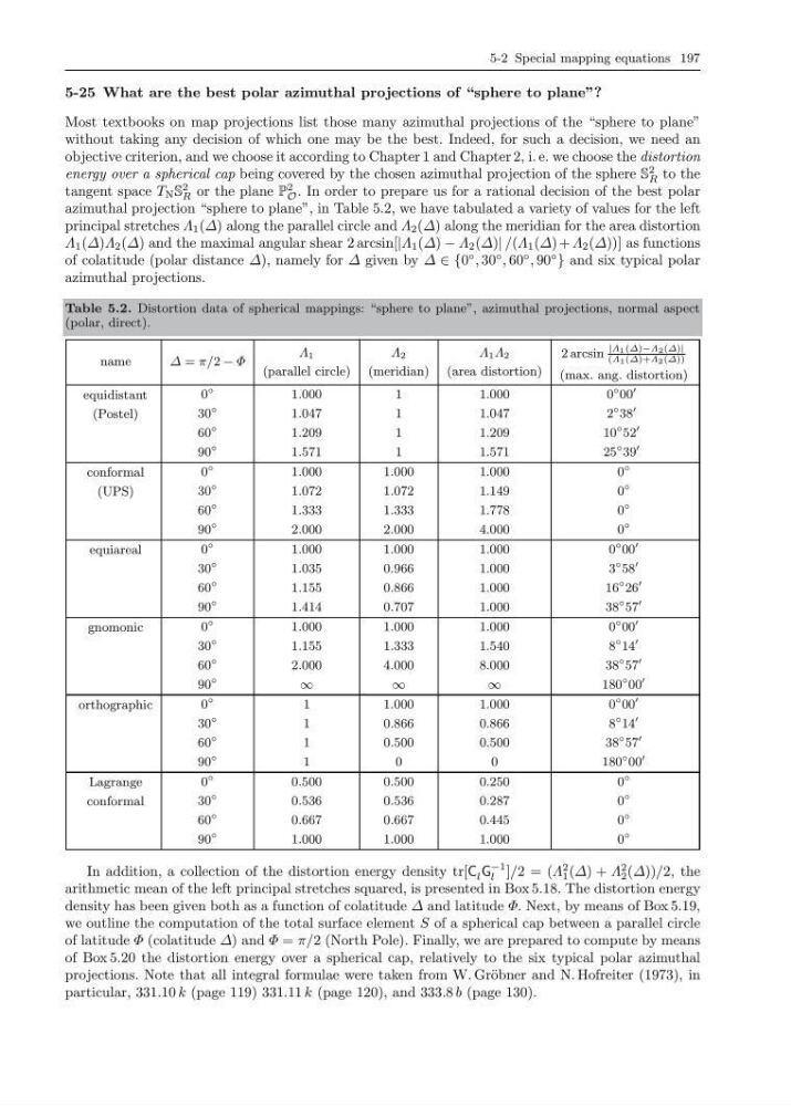
azimuthal projection “sphere to plane”, in Table 5.2, we have tabulated a variety of values for the left
principal stretches Λ 1 (∆) along the parallel circle and Λ 2 (∆) along the meridian for the area distortion
Λ 1 (∆)Λ 2 (∆) and the maximal angular shear 2 arcsin[|Λ 1 (∆) − Λ 2 (∆)| /(Λ 1 (∆) + Λ 2 (∆))] as functions
of colatitude (polar distance ∆), namely for ∆ given by ∆ ∈ {0
◦ , 30
◦ , 60
◦ , 90
◦
} and six typical polar
azimuthal projections.
Table 5.2. Distortion data of spherical mappings: “sphere to plane”, azimuthal projections, normal aspect
(polar, direct).
name
∆ = π/2 − Φ
Λ 1
(parallel circle)
Λ 2
(meridian)
Λ 1 Λ 2
(area distortion)
2 arcsin
|Λ 1 (∆)−Λ 2 (∆)|
(Λ 1 (∆)+Λ 2 (∆))
(max. ang. distortion)
equidistant
0
◦
1.000
1
1.000
0
◦ 00
(Postel)
30
◦
1.047
1
1.047
2
◦ 38
60
◦
1.209
1
1.209
10
◦ 52
90
◦
1.571
1
1.571
25
◦ 39
conformal
0
◦
1.000
1.000
1.000
0
◦
(UPS)
30
◦
1.072
1.072
1.149
0
◦
60
◦
1.333
1.333
1.778
0
◦
90
◦
2.000
2.000
4.000
0
◦
equiareal
0
◦
1.000
1.000
1.000
0
◦ 00
30
◦
1.035
0.966
1.000
3
◦ 58
60
◦
1.155
0.866
1.000
16
◦ 26
90
◦
1.414
0.707
1.000
38
◦ 57
gnomonic
0
◦
1.000
1.000
1.000
0
◦ 00
30
◦
1.155
1.333
1.540
8
◦ 14
60
◦
2.000
4.000
8.000
38
◦ 57
90
◦
∞
∞
∞
180
◦ 00
orthographic
0
◦
1
1.000
1.000
0
◦ 00
30
◦
1
0.866
0.866
8
◦ 14
60
◦
1
0.500
0.500
38
◦ 57
90
◦
1
0
0
180
◦ 00
Lagrange
0
◦
0.500
0.500
0.250
0
◦
conformal
30
◦
0.536
0.536
0.287
0
◦
60
◦
0.667
0.667
0.445
0
◦
90
◦
1.000
1.000
1.000
0
◦
In addition, a collection of the distortion energy density tr[C l G
−1
l ]/2 = (Λ
2
1 (∆) + Λ
2
2 (∆))/2, the
arithmetic mean of the left principal stretches squared, is presented in Box 5.18. The distortion energy
density has been given both as a function of colatitude ∆ and latitude Φ. Next, by means of Box 5.19,
we outline the computation of the total surface element S of a spherical cap between a parallel circle
of latitude Φ (colatitude ∆) and Φ = π/2 (North Pole). Finally, we are prepared to compute by means
of Box 5.20 the distortion energy over a spherical cap, relatively to the six typical polar azimuthal
projections. Note that all integral formulae were taken from W. Gr¨ obner and N. Hofreiter (1973), in
particular, 331.10 k (page 119) 331.11 k (page 120), and 333.8 b (page 130).
5-25 What are the best polar azimuthal projections of “sphere to plane”?
Most textbooks on map projections list those many azimuthal projections of the “sphere to plane”
without taking any decision of which one may be the best. Indeed, for such a decision, we need an
objective criterion, and we choose it according to Chapter 1 and Chapter 2, i. e. we choose the distortion
energy over a spherical cap being covered by the chosen azimuthal projection of the sphere S
2
R to the
tangent space T N S
2
R or the plane P
2
O . In order to prepare us for a rational decision of the best polar
azimuthal projection “sphere to plane”, in Table 5.2, we have tabulated a variety of values for the left
principal stretches Λ 1 (∆) along the parallel circle and Λ 2 (∆) along the meridian for the area distortion
Λ 1 (∆)Λ 2 (∆) and the maximal angular shear 2 arcsin[|Λ 1 (∆) − Λ 2 (∆)| /(Λ 1 (∆) + Λ 2 (∆))] as functions
of colatitude (polar distance ∆), namely for ∆ given by ∆ ∈ {0
◦ , 30
◦ , 60
◦ , 90
◦
} and six typical polar
azimuthal projections.
Table 5.2. Distortion data of spherical mappings: “sphere to plane”, azimuthal projections, normal aspect
(polar, direct).
name
∆ = π/2 − Φ
Λ 1
(parallel circle)
Λ 2
(meridian)
Λ 1 Λ 2
(area distortion)
2 arcsin
|Λ 1 (∆)−Λ 2 (∆)|
(Λ 1 (∆)+Λ 2 (∆))
(max. ang. distortion)
equidistant
0
◦
1.000
1
1.000
0
◦ 00
(Postel)
30
◦
1.047
1
1.047
2
◦ 38
60
◦
1.209
1
1.209
10
◦ 52
90
◦
1.571
1
1.571
25
◦ 39
conformal
0
◦
1.000
1.000
1.000
0
◦
(UPS)
30
◦
1.072
1.072
1.149
0
◦
60
◦
1.333
1.333
1.778
0
◦
90
◦
2.000
2.000
4.000
0
◦
equiareal
0
◦
1.000
1.000
1.000
0
◦ 00
30
◦
1.035
0.966
1.000
3
◦ 58
60
◦
1.155
0.866
1.000
16
◦ 26
90
◦
1.414
0.707
1.000
38
◦ 57
gnomonic
0
◦
1.000
1.000
1.000
0
◦ 00
30
◦
1.155
1.333
1.540
8
◦ 14
60
◦
2.000
4.000
8.000
38
◦ 57
90
◦
∞
∞
∞
180
◦ 00
orthographic
0
◦
1
1.000
1.000
0
◦ 00
30
◦
1
0.866
0.866
8
◦ 14
60
◦
1
0.500
0.500
38
◦ 57
90
◦
1
0
0
180
◦ 00
Lagrange
0
◦
0.500
0.500
0.250
0
◦
conformal
30
◦
0.536
0.536
0.287
0
◦
60
◦
0.667
0.667
0.445
0
◦
90
◦
1.000
1.000
1.000
0
◦
In addition, a collection of the distortion energy density tr[C l G
−1
l ]/2 = (Λ
2
1 (∆) + Λ
2
2 (∆))/2, the
arithmetic mean of the left principal stretches squared, is presented in Box 5.18. The distortion energy
density has been given both as a function of colatitude ∆ and latitude Φ. Next, by means of Box 5.19,
we outline the computation of the total surface element S of a spherical cap between a parallel circle
of latitude Φ (colatitude ∆) and Φ = π/2 (North Pole). Finally, we are prepared to compute by means
of Box 5.20 the distortion energy over a spherical cap, relatively to the six typical polar azimuthal
projections. Note that all integral formulae were taken from W. Gr¨ obner and N. Hofreiter (1973), in
particular, 331.10 k (page 119) 331.11 k (page 120), and 333.8 b (page 130).