5-1 General mapping equations 165
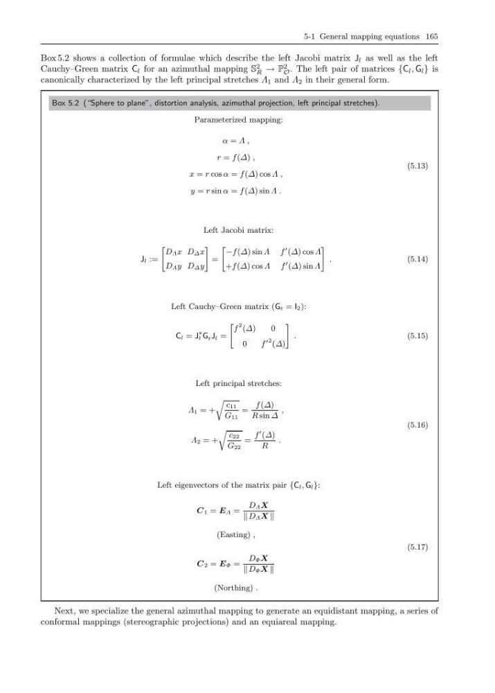
Box 5.2 shows a collection of formulae which describe the left Jacobi matrix J l as well as the left
Cauchy–Green matrix C l for an azimuthal mapping S
2
R → P
2
O . The left pair of matrices {C l , G l } is
canonically characterized by the left principal stretches Λ 1 and Λ 2 in their general form.
Box 5.2 (“Sphere to plane”, distortion analysis, azimuthal projection, left principal stretches).
Parameterized mapping:
α = Λ ,
r = f (∆) ,
x = r cos α = f (∆) cos Λ ,
y = r sin α = f (∆) sin Λ .
(5.13)
Left Jacobi matrix:
J l :=
"
D Λ x D ∆ x
D Λ y D ∆ y
#
=
" −f (∆) sin Λ f
(∆) cos Λ
+f (∆) cos Λ f
(∆) sin Λ
#
.
(5.14)
Left Cauchy–Green matrix (G r = I 2 ):
C l = J
∗
l G r J l =
"
f
2 (∆)
0
0
f
2 (∆)
#
.
(5.15)
Left principal stretches:
Λ 1 = +
r
c 11
G 11
=
f (∆)
R sin ∆
,
Λ 2 = +
r
c 22
G 22
=
f
(∆)
R
.
(5.16)
Left eigenvectors of the matrix pair {C l , G l }:
C 1 = E Λ =
D Λ X
D Λ X
(Easting) ,
C 2 = E Φ =
D Φ X
D Φ X
(Northing) .
(5.17)
Next, we specialize the general azimuthal mapping to generate an equidistant mapping, a series of
conformal mappings (stereographic projections) and an equiareal mapping.