

3-4 The oblique frame of reference of the ellipsoid-of-revolution 149
Let us here additionally collect the result of the transformation {A, B} → {Λ, Φ} by the following
Corollary 3.9.
Corollary 3.9 (The change from one chart to another chart: cha-cha-cha, the oblique quasi-spherical
longitude/latitude versus the surface normal ellipsoidal longitude/latitude).
Given the longitude of the ascending node Ω as well as the inclination I of the oblique equatorial plane,
then the transformation of oblique quasi-spherical longitude/latitude in surface normal ellipsoidal
longitude/latitude is represented by (3.133).
End of Corollary.
Next, let us assume that we know already a point {Λ 0 , Φ 0 }, correspondingly {A 0 , B 0 }, in E
2
A 1 ,A 2
.
Relative to such a fixed point, we are able to find the coordinates {Λ, Φ}, correspondingly {A, B},
close to {Λ 0 , Φ 0 }, correspondingly {A 0 , B 0 }, by a Taylor series expansion of the type presented in
Boxes 3.20 and 3.21.
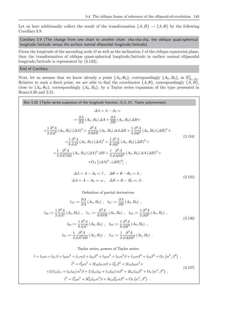
Box 3.20 (Taylor series expansion of the longitude function Λ(A, B), Taylor polynomials).
∆Λ = Λ − Λ 0 =
=
∂Λ
∂A
(A 0 , B 0 ) ∆A +
∂Λ
∂B
(A 0 , B 0 ) ∆B+
+
1
2
∂
2 Λ
∂A
2 (A 0 , B 0 ) (∆A)
2 +
∂
2 Λ
∂A∂B
(A 0 , B 0 ) ∆A∆B +
1
2
∂
2 Λ
∂B
2 (A 0 , B 0 ) (∆B)
2 +
+
1
6
∂
3 Λ
∂A
3 (A 0 , B 0 ) (∆A)
3 +
1
6
∂
3 Λ
∂B
3 (A 0 , B 0 ) (∆B)
3 +
+
1
2
∂
3 Λ
∂A
2 ∂B
(A 0 , B 0 ) (∆A)
2 ∆B +
1
2
∂
3 Λ
∂A∂B
2 (A 0 , B 0 ) ∆A (∆B)
2 +
+O Λ
ˆ
(∆A)
4 , (∆B)
4 ˜
,
(3.134)
∆Λ = Λ − Λ 0 =: l , ∆Φ = Φ − Φ 0 =: b ,
∆A = A − A 0 =: α , ∆B = B − B 0 =: β .
(3.135)
Definition of partial derivatives:
l 10 :=
∂Λ
∂A
(A 0 , B 0 ) , l 01 :=
∂Λ
∂B
(A 0 , B 0 ) ,
l 20 :=
1
2
∂
2 Λ
∂A
2 (A 0 , B 0 ) , l 11 :=
∂
2 Λ
∂A∂B
(A 0 , B 0 ) , l 02 :=
1
2
∂
2 Λ
∂B
2 (A 0 , B 0 ) ,
l 30 :=
1
6
∂
3 Λ
∂A
3 (A 0 , B 0 ) , l 03 :=
1
6
∂
3 Λ
∂B
3 (A 0 , B 0 ) ,
l 21 :=
1
2
∂
3 Λ
∂A
2 ∂B
(A 0 , B 0 ) , l 12 :=
1
2
∂
3 Λ
∂A∂B
2 (A 0 , B 0 ) .
(3.136)
Taylor series, powers of Taylor series:
l = l 10 α + l 01 β + l 20 α
2 + l 11 αβ + l 02 β
2 + l 30 α
3 + l 21 α
2 β + l 12 αβ
2 + l 03 β
3 + O 1
`
α
4 , β
4 ´
,
l
2 = l
2
10 α
2 + 2l 10 l 01 αβ + l
2
01 β
2 + 2l 10 l 20 α
3 +
+2 (l 10 l 11 + l 01 l 20 ) α
2 β + 2 (l 01 l 20 + l 10 l 02 ) αβ
2 + 2l 01 l 02 β
3 + O 2
`
α
4 , β
4 ´
,
l
3 = l
3
10 α
3 + 3l
2
10 l 01 α
2 β + 3l 10 l
2
01 αβ
2 + O 3
`
α
4 , β
4 ´
.
(3.137)
Let us here additionally collect the result of the transformation {A, B} → {Λ, Φ} by the following
Corollary 3.9.
Corollary 3.9 (The change from one chart to another chart: cha-cha-cha, the oblique quasi-spherical
longitude/latitude versus the surface normal ellipsoidal longitude/latitude).
Given the longitude of the ascending node Ω as well as the inclination I of the oblique equatorial plane,
then the transformation of oblique quasi-spherical longitude/latitude in surface normal ellipsoidal
longitude/latitude is represented by (3.133).
End of Corollary.
Next, let us assume that we know already a point {Λ 0 , Φ 0 }, correspondingly {A 0 , B 0 }, in E
2
A 1 ,A 2
.
Relative to such a fixed point, we are able to find the coordinates {Λ, Φ}, correspondingly {A, B},
close to {Λ 0 , Φ 0 }, correspondingly {A 0 , B 0 }, by a Taylor series expansion of the type presented in
Boxes 3.20 and 3.21.
Box 3.20 (Taylor series expansion of the longitude function Λ(A, B), Taylor polynomials).
∆Λ = Λ − Λ 0 =
=
∂Λ
∂A
(A 0 , B 0 ) ∆A +
∂Λ
∂B
(A 0 , B 0 ) ∆B+
+
1
2
∂
2 Λ
∂A
2 (A 0 , B 0 ) (∆A)
2 +
∂
2 Λ
∂A∂B
(A 0 , B 0 ) ∆A∆B +
1
2
∂
2 Λ
∂B
2 (A 0 , B 0 ) (∆B)
2 +
+
1
6
∂
3 Λ
∂A
3 (A 0 , B 0 ) (∆A)
3 +
1
6
∂
3 Λ
∂B
3 (A 0 , B 0 ) (∆B)
3 +
+
1
2
∂
3 Λ
∂A
2 ∂B
(A 0 , B 0 ) (∆A)
2 ∆B +
1
2
∂
3 Λ
∂A∂B
2 (A 0 , B 0 ) ∆A (∆B)
2 +
+O Λ
ˆ
(∆A)
4 , (∆B)
4 ˜
,
(3.134)
∆Λ = Λ − Λ 0 =: l , ∆Φ = Φ − Φ 0 =: b ,
∆A = A − A 0 =: α , ∆B = B − B 0 =: β .
(3.135)
Definition of partial derivatives:
l 10 :=
∂Λ
∂A
(A 0 , B 0 ) , l 01 :=
∂Λ
∂B
(A 0 , B 0 ) ,
l 20 :=
1
2
∂
2 Λ
∂A
2 (A 0 , B 0 ) , l 11 :=
∂
2 Λ
∂A∂B
(A 0 , B 0 ) , l 02 :=
1
2
∂
2 Λ
∂B
2 (A 0 , B 0 ) ,
l 30 :=
1
6
∂
3 Λ
∂A
3 (A 0 , B 0 ) , l 03 :=
1
6
∂
3 Λ
∂B
3 (A 0 , B 0 ) ,
l 21 :=
1
2
∂
3 Λ
∂A
2 ∂B
(A 0 , B 0 ) , l 12 :=
1
2
∂
3 Λ
∂A∂B
2 (A 0 , B 0 ) .
(3.136)
Taylor series, powers of Taylor series:
l = l 10 α + l 01 β + l 20 α
2 + l 11 αβ + l 02 β
2 + l 30 α
3 + l 21 α
2 β + l 12 αβ
2 + l 03 β
3 + O 1
`
α
4 , β
4 ´
,
l
2 = l
2
10 α
2 + 2l 10 l 01 αβ + l
2
01 β
2 + 2l 10 l 20 α
3 +
+2 (l 10 l 11 + l 01 l 20 ) α
2 β + 2 (l 01 l 20 + l 10 l 02 ) αβ
2 + 2l 01 l 02 β
3 + O 2
`
α
4 , β
4 ´
,
l
3 = l
3
10 α
3 + 3l
2
10 l 01 α
2 β + 3l 10 l
2
01 αβ
2 + O 3
`
α
4 , β
4 ´
.
(3.137)