

122 3 Coordinates
x
y
x
e1
e2
λ p
p = π 1 (P )
P
0
2 π
0 < λ < 2π
y
= −x
x
= y
x
e 2
e 1
α
q
q = π 2 (P )
P
0
2 π
0 < α < 2π
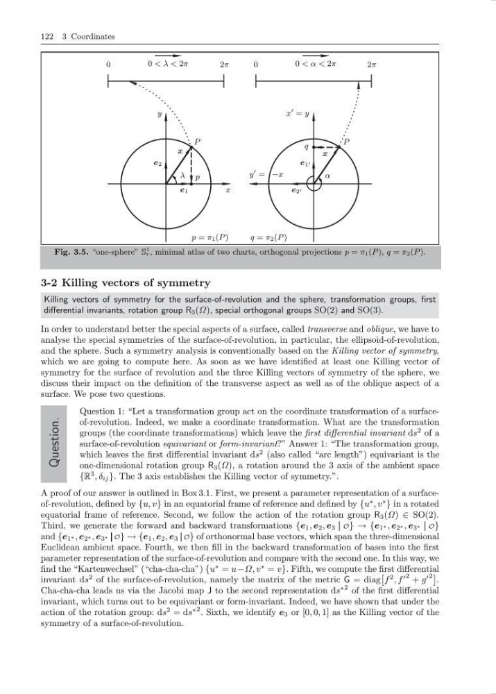
Fig. 3.5. “one-sphere” S
1
r , minimal atlas of two charts, orthogonal projections p = π 1 (P ), q = π 2 (P ).
3-2 Killing vectors of symmetry
Killing vectors of symmetry for the surface-of-revolution and the sphere, transformation groups, first
differential invariants, rotation group R 3 (Ω), special orthogonal groups SO(2) and SO(3).
In order to understand better the special aspects of a surface, called transverse and oblique, we have to
analyse the special symmetries of the surface-of-revolution, in particular, the ellipsoid-of-revolution,
and the sphere. Such a symmetry analysis is conventionally based on the Killing vector of symmetry,
which we are going to compute here. As soon as we have identified at least one Killing vector of
symmetry for the surface of revolution and the three Killing vectors of symmetry of the sphere, we
discuss their impact on the definition of the transverse aspect as well as of the oblique aspect of a
surface. We pose two questions.
Question.
Question 1: “Let a transformation group act on the coordinate transformation of a surfaceof-revolution. Indeed, we make a coordinate transformation. What are the transformation
groups (the coordinate transformations) which leave the first differential invariant ds
2 of a
surface-of-revolution equivariant or form-invariant?” Answer 1: “The transformation group,
which leaves the first differential invariant ds
2 (also called “arc length”) equivariant is the
one-dimensional rotation group R 3 (Ω), a rotation around the 3 axis of the ambient space
{R
3 , δ ij }. The 3 axis establishes the Killing vector of symmetry.”.
A proof of our answer is outlined in Box 3.1. First, we present a parameter representation of a surfaceof-revolution, defined by {u, v} in an equatorial frame of reference and defined by {u
∗ , v
∗
} in a rotated
equatorial frame of reference. Second, we follow the action of the rotation group R 3 (Ω) ∈ SO(2).
Third, we generate the forward and backward transformations {e 1 , e 2 , e 3 O} → {e 1 ∗ , e 2 ∗ , e 3 ∗ O}
and {e 1 ∗ , e 2 ∗ , e 3 ∗ O} → {e 1 , e 2 , e 3 O} of orthonormal base vectors, which span the three-dimensional
Euclidean ambient space. Fourth, we then fill in the backward transformation of bases into the first
parameter representation of the surface-of-revolution and compare with the second one. In this way, we
find the “Kartenwechsel” (“cha-cha-cha”) {u
∗ = u−Ω, v
∗ = v}. Fifth, we compute the first differential
invariant ds
2 of the surface-of-revolution, namely the matrix of the metric G = diag
f
2 , f
2 + g
2
.
Cha-cha-cha leads us via the Jacobi map J to the second representation ds
∗2 of the first differential
invariant, which turns out to be equivariant or form-invariant. Indeed, we have shown that under the
action of the rotation group: ds
2 = ds
∗2 . Sixth, we identify e 3 or [0, 0, 1] as the Killing vector of the
symmetry of a surface-of-revolution.
x
y
x
e1
e2
λ p
p = π 1 (P )
P
0
2 π
0 < λ < 2π
y
= −x
x
= y
x
e 2
e 1
α
q
q = π 2 (P )
P
0
2 π
0 < α < 2π
Fig. 3.5. “one-sphere” S
1
r , minimal atlas of two charts, orthogonal projections p = π 1 (P ), q = π 2 (P ).
3-2 Killing vectors of symmetry
Killing vectors of symmetry for the surface-of-revolution and the sphere, transformation groups, first
differential invariants, rotation group R 3 (Ω), special orthogonal groups SO(2) and SO(3).
In order to understand better the special aspects of a surface, called transverse and oblique, we have to
analyse the special symmetries of the surface-of-revolution, in particular, the ellipsoid-of-revolution,
and the sphere. Such a symmetry analysis is conventionally based on the Killing vector of symmetry,
which we are going to compute here. As soon as we have identified at least one Killing vector of
symmetry for the surface of revolution and the three Killing vectors of symmetry of the sphere, we
discuss their impact on the definition of the transverse aspect as well as of the oblique aspect of a
surface. We pose two questions.
Question.
Question 1: “Let a transformation group act on the coordinate transformation of a surfaceof-revolution. Indeed, we make a coordinate transformation. What are the transformation
groups (the coordinate transformations) which leave the first differential invariant ds
2 of a
surface-of-revolution equivariant or form-invariant?” Answer 1: “The transformation group,
which leaves the first differential invariant ds
2 (also called “arc length”) equivariant is the
one-dimensional rotation group R 3 (Ω), a rotation around the 3 axis of the ambient space
{R
3 , δ ij }. The 3 axis establishes the Killing vector of symmetry.”.
A proof of our answer is outlined in Box 3.1. First, we present a parameter representation of a surfaceof-revolution, defined by {u, v} in an equatorial frame of reference and defined by {u
∗ , v
∗
} in a rotated
equatorial frame of reference. Second, we follow the action of the rotation group R 3 (Ω) ∈ SO(2).
Third, we generate the forward and backward transformations {e 1 , e 2 , e 3 O} → {e 1 ∗ , e 2 ∗ , e 3 ∗ O}
and {e 1 ∗ , e 2 ∗ , e 3 ∗ O} → {e 1 , e 2 , e 3 O} of orthonormal base vectors, which span the three-dimensional
Euclidean ambient space. Fourth, we then fill in the backward transformation of bases into the first
parameter representation of the surface-of-revolution and compare with the second one. In this way, we
find the “Kartenwechsel” (“cha-cha-cha”) {u
∗ = u−Ω, v
∗ = v}. Fifth, we compute the first differential
invariant ds
2 of the surface-of-revolution, namely the matrix of the metric G = diag
f
2 , f
2 + g
2
.
Cha-cha-cha leads us via the Jacobi map J to the second representation ds
∗2 of the first differential
invariant, which turns out to be equivariant or form-invariant. Indeed, we have shown that under the
action of the rotation group: ds
2 = ds
∗2 . Sixth, we identify e 3 or [0, 0, 1] as the Killing vector of the
symmetry of a surface-of-revolution.