

78
4. Finite Difference Methods
is satisfied, then in terms of Eq. (4.1.23), we can obtain the estimation:
E"+1 :s;; DE" + (1 - 2D - V)E" + (D + V)E" + O[(L\t)2 + L\t· L\x]
= E" + O[(L\t)2 + L\t. L\x]
(4.1.25)
where E,,+! and E" are used to indicate the maximum absolute values of e at
time levels n + 1 and n, respectively. Since the initial condition used in the
difference equation is the same as in the original equation, we have E o = o.
Thus, from Eq. (4.1.25), we have
EI :s;; O[(L\t)2 + L\t· L\x]
E 2 :S;; 2· o [(L\t)2 + L\t·L\x]
These equations show that E" -+ 0 as long as L\t -+ 0, L\x -+ 0 at any time level
n. They also show that the solutions of the difference equations tend to the
exact solution of the differential equation at the nodes, if condition (4.1.24) is
satisfied. Substituting Eq. (4.1.22) into Eq. (4.1.24), we obtain:
2DL\t VL\t _ L\ 2D + VL\x 1
(L\X)2 + L\x - t (L\X)2 <,
which isjust the condition given in Eq. (4.1.19). The error-enlargement factor
ofthe difference equation from one time level to the next can be calculated by
von Neumann's stability analysis, we have,
{(
DL\t
ßL\t)2 (VL\t)2
} 1/2
lei = 1 - 4 (L\X)2 sin 2 L\x + L\x sin
2
ßL\t
.
(4.1.26)
A detailed analysis of the convergence and stability of various difference
schemes can be found in the book written by Lapidus and Pinder (1982).
For the one-dimensional advection-dispersion equation with a variable
dispersion coefficient:
oC _ ° (D oC ) VoC
fu - ox ox - ox'
(4.1.27)
we can use the following difference formula
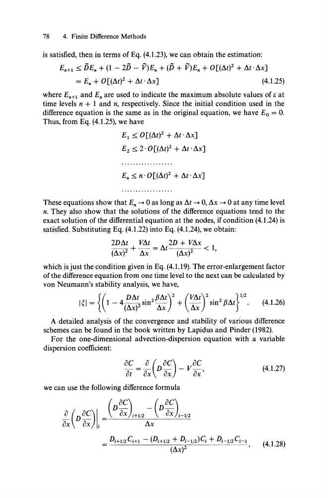
(4.1.28)
4. Finite Difference Methods
is satisfied, then in terms of Eq. (4.1.23), we can obtain the estimation:
E"+1 :s;; DE" + (1 - 2D - V)E" + (D + V)E" + O[(L\t)2 + L\t· L\x]
= E" + O[(L\t)2 + L\t. L\x]
(4.1.25)
where E,,+! and E" are used to indicate the maximum absolute values of e at
time levels n + 1 and n, respectively. Since the initial condition used in the
difference equation is the same as in the original equation, we have E o = o.
Thus, from Eq. (4.1.25), we have
EI :s;; O[(L\t)2 + L\t· L\x]
E 2 :S;; 2· o [(L\t)2 + L\t·L\x]
These equations show that E" -+ 0 as long as L\t -+ 0, L\x -+ 0 at any time level
n. They also show that the solutions of the difference equations tend to the
exact solution of the differential equation at the nodes, if condition (4.1.24) is
satisfied. Substituting Eq. (4.1.22) into Eq. (4.1.24), we obtain:
2DL\t VL\t _ L\ 2D + VL\x 1
(L\X)2 + L\x - t (L\X)2 <,
which isjust the condition given in Eq. (4.1.19). The error-enlargement factor
ofthe difference equation from one time level to the next can be calculated by
von Neumann's stability analysis, we have,
{(
DL\t
ßL\t)2 (VL\t)2
} 1/2
lei = 1 - 4 (L\X)2 sin 2 L\x + L\x sin
2
ßL\t
.
(4.1.26)
A detailed analysis of the convergence and stability of various difference
schemes can be found in the book written by Lapidus and Pinder (1982).
For the one-dimensional advection-dispersion equation with a variable
dispersion coefficient:
oC _ ° (D oC ) VoC
fu - ox ox - ox'
(4.1.27)
we can use the following difference formula
(4.1.28)