

64
3. Analytic Solutions of Hydrodynamic Dispersion Equations
Problem 5. Two- and Three-dimensional Dispersions of a Tracer in a
Semi-infinite Region
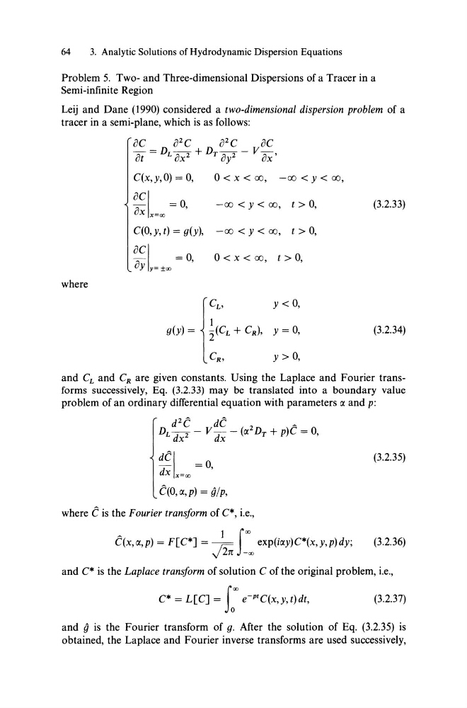
Leij and Dane (1990) considered a two-dimensional dispersion problem of a
tracer in a semi-plane, which is as follows:
C(x, y, 0) = 0,
° < x < 00, -00 < y < 00,
OCI =0
ox x=oo '
-00 < y < 00, t > 0,
(3.2.33)
C(O, y, t) = g(y), -00 < y < 00, t > 0,
~~ Iy= ±oo = 0, ° < x < 00, t > 0,
where
g(y) =
1
2(CL + CR)' y = 0,
(3.2.34)
CR'
Y > 0,
and CL and C R are given constants. Using the Laplace and Fourier transforms successively, Eq. (3.2.33) may be translated into a boundary value
problem of an ordinary differential equation with parameters 0( and p:
2 ~
~
d C
dC
2
~
DL dx2 - V dx - (0( DT + p)C = 0,
dCI =0
dx x=oo '
(3.2.35)
C(O, 0(, p) = O/p,
where Cis the Fourier transform of C*, i.e.,
~
1 Joo
C(x,O(,p) = F[C*] = M:
exp(iO(y)C*(x,y,p)dy;
v 2n -00
(3.2.36)
and C* is the Laplace transform of solution C of the original problem, i.e.,
C* = L[C] = Ioo e-PtC(x,y,t)dt,
(3.2.37)
and 0 is the Fourier transform of g. After the solution of Eq. (3.2.35) is
obtained, the Laplace and Fourier inverse transforms are used successively,
3. Analytic Solutions of Hydrodynamic Dispersion Equations
Problem 5. Two- and Three-dimensional Dispersions of a Tracer in a
Semi-infinite Region
Leij and Dane (1990) considered a two-dimensional dispersion problem of a
tracer in a semi-plane, which is as follows:
C(x, y, 0) = 0,
° < x < 00, -00 < y < 00,
OCI =0
ox x=oo '
-00 < y < 00, t > 0,
(3.2.33)
C(O, y, t) = g(y), -00 < y < 00, t > 0,
~~ Iy= ±oo = 0, ° < x < 00, t > 0,
where
g(y) =
1
2(CL + CR)' y = 0,
(3.2.34)
CR'
Y > 0,
and CL and C R are given constants. Using the Laplace and Fourier transforms successively, Eq. (3.2.33) may be translated into a boundary value
problem of an ordinary differential equation with parameters 0( and p:
2 ~
~
d C
dC
2
~
DL dx2 - V dx - (0( DT + p)C = 0,
dCI =0
dx x=oo '
(3.2.35)
C(O, 0(, p) = O/p,
where Cis the Fourier transform of C*, i.e.,
~
1 Joo
C(x,O(,p) = F[C*] = M:
exp(iO(y)C*(x,y,p)dy;
v 2n -00
(3.2.36)
and C* is the Laplace transform of solution C of the original problem, i.e.,
C* = L[C] = Ioo e-PtC(x,y,t)dt,
(3.2.37)
and 0 is the Fourier transform of g. After the solution of Eq. (3.2.35) is
obtained, the Laplace and Fourier inverse transforms are used successively,