

8.1. Simulation and Prediction of Groundwater Pollution
255
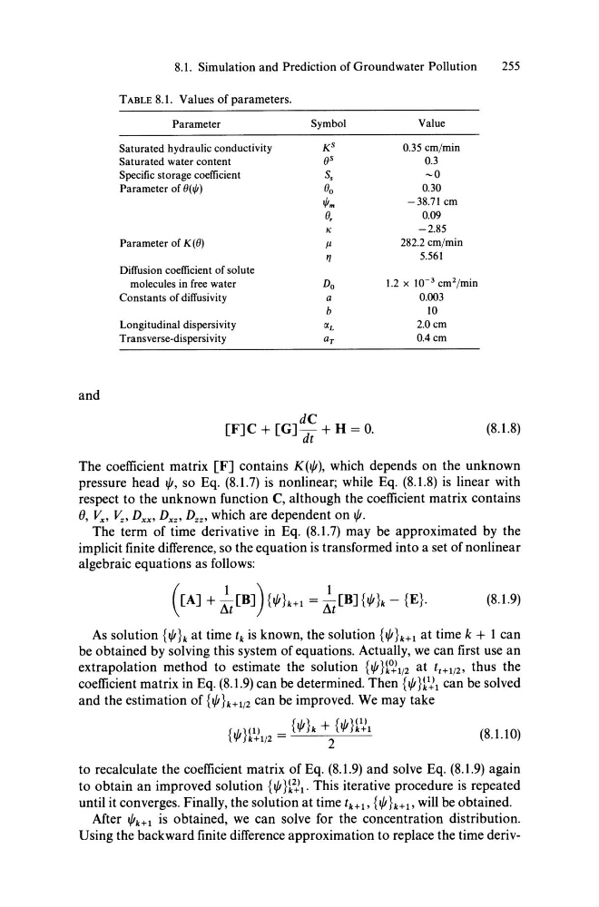
T ABLE 8.1. Values of parameters.
Parameter
Symbol
Value
Saturated hydraulic conductivity
K S
0.35 cmjmin
Saturated water content
Os
0.3
Specific storage coefficient
S,
-0
Parameter of O(l/I)
00
0.30
l/Im
-38.71 cm
0,
0.09
K
-2.85
Parameter of K(O)
Il
282.2 cmjmin
"
5.561
Diffusion coefficient of solute
moleeules in free water
Do
1.2 x 10- 3 cm 2 jmin
Constants of diffusivity
a
0.003
b
10
Longitudinal dispersivity
C(L
2.0cm
Transverse-dispersivity
aT
0.4cm
and
dC
[F]C + [Gl Tt + H = O.
(8.1.8)
The coefficient matrix [F] contains K(I/I), which depends on the unknown
pressure head 1/1, so Eq. (8.1.7) is nonlinear; while Eq. (8.1.8) is linear with
respect to the unknown function C, although the coefficient matrix contains
8, Vx , Y." Dxx' Dxz , Dzz> wh ich are dependent on 1/1.
The term of time derivative in Eq. (8.1.7) may be approximated by the
implicit finite difference, so the equation is transformed into a set of nonlinear
algebraic equations as folIows:
([A] + ~t[B]){I/Ih+1 = ~t[BJ{I/Ih - {E}.
(8.1.9)
As solution {I/I h at time tk is known, the solution {I/I h+1 at time k + 1 can
be obtained by solving this system of equations. Actually, we can first use an
extrapolation method to estimate the solution {I/I H~1/2 at tl +1 /2 , thus the
coefficient matrix in Eq. (8.1.9) can be determined. Then {I/I H~l can be solved
and the estimation of {I/Ih+1/2 can be improved. We may take
{I/IH~1/2 = {I/I}k +2{I/IH~1
(8.1.10)
to recalculate the coefficient matrix of Eq. (8.1.9) and solve Eq. (8.1.9) again
to obtain an improved solution {I/I W21' This iterative procedure is repeated
until it converges. Finally, the solution at time tk+1' {I/I h+1' will be obtained.
After I/Ik+1 is obtained, we can solve for the concentration distribution.
Using the back ward finite difference approximation to replace the time deriv-
255
T ABLE 8.1. Values of parameters.
Parameter
Symbol
Value
Saturated hydraulic conductivity
K S
0.35 cmjmin
Saturated water content
Os
0.3
Specific storage coefficient
S,
-0
Parameter of O(l/I)
00
0.30
l/Im
-38.71 cm
0,
0.09
K
-2.85
Parameter of K(O)
Il
282.2 cmjmin
"
5.561
Diffusion coefficient of solute
moleeules in free water
Do
1.2 x 10- 3 cm 2 jmin
Constants of diffusivity
a
0.003
b
10
Longitudinal dispersivity
C(L
2.0cm
Transverse-dispersivity
aT
0.4cm
and
dC
[F]C + [Gl Tt + H = O.
(8.1.8)
The coefficient matrix [F] contains K(I/I), which depends on the unknown
pressure head 1/1, so Eq. (8.1.7) is nonlinear; while Eq. (8.1.8) is linear with
respect to the unknown function C, although the coefficient matrix contains
8, Vx , Y." Dxx' Dxz , Dzz> wh ich are dependent on 1/1.
The term of time derivative in Eq. (8.1.7) may be approximated by the
implicit finite difference, so the equation is transformed into a set of nonlinear
algebraic equations as folIows:
([A] + ~t[B]){I/Ih+1 = ~t[BJ{I/Ih - {E}.
(8.1.9)
As solution {I/I h at time tk is known, the solution {I/I h+1 at time k + 1 can
be obtained by solving this system of equations. Actually, we can first use an
extrapolation method to estimate the solution {I/I H~1/2 at tl +1 /2 , thus the
coefficient matrix in Eq. (8.1.9) can be determined. Then {I/I H~l can be solved
and the estimation of {I/Ih+1/2 can be improved. We may take
{I/IH~1/2 = {I/I}k +2{I/IH~1
(8.1.10)
to recalculate the coefficient matrix of Eq. (8.1.9) and solve Eq. (8.1.9) again
to obtain an improved solution {I/I W21' This iterative procedure is repeated
until it converges. Finally, the solution at time tk+1' {I/I h+1' will be obtained.
After I/Ik+1 is obtained, we can solve for the concentration distribution.
Using the back ward finite difference approximation to replace the time deriv-