

8.1. Simulation and Prediction ofGroundwater Pollution
253
In the third stage, a water quality model was built. The simulated area was
168 km 2 , located in the northern suburb of Xi'an, and was divided into 307
triangular elements. The two-dimensional advection-dispersion model was
selected as the simulation model. The upstream weighted multiple cell balance method was used to avoid the oscillation of numerical solutions. The
parameters to be identified in the model inc1uding longitudinal dispersivity
Il L , transverse dispersivity Il T , and the amount of irrigation return water
in the sewage irrigation area. The model outputs were compared with the
observed concentration data in 25 years (1959 to 1984) and unknown parameters were adjusted based on the comparison. Finally, a good fit was reached,
where IlL and IlT were determined to be about 130 m and 48 m, respectively.
In the fourth stage, the calibrated model was used for prediction. Several
possible projects of reducing groundwater pollution were simulated.
There are many things in common in the groundwater pollution research
between the Xi'an City and the munitions factory in Colorado. In both cases,
chloride ion was used as the tracer and long-term observation data was used
to calibrate the flow model and water quality model. However, the aquifer of
the Xi'an City consists of a larger area with more complex conditions.
8.1.3 Groundwater Pollution of Saturated-Unsaturated
Aquifers
It is very important to study the solute transport in unsaturated zones. In
practice, however, the use of the mathematical models is still very difficult
owing to the non-linearity of the problem. In particular, it is difficult to
obtain the input parameters. Advection-dispersion models ofwater quality in
the saturated-unsaturated zone have been introduced in Section 7.1.2. For
instance, a two-dimensional problem of a profile is governed by the following
water flow equation
«( + PS.) ~~ = :x [ K(ifJ) ~~ ] + :z [ K(ifJ) ~~ ] + :z K(ifJ) + W, (8.1.1)
and the water quality equation
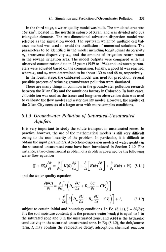
(8.1.2)
subject to certain initial and boundary conditions. In Eq. (8.1.1), ( = oO/oifJ;
o is the soil moisture content; ifJ is the pressure water head; P is equal to 1 in
the saturated zone and 0 in the unsaturated zone, and K(ifJ) is the hydraulic
conductivity in the saturated-unsaturated zone. In Eq. (8.1.2), the sink/source
term, I, may contain the radioactive decay, adsorption, chemical re action
253
In the third stage, a water quality model was built. The simulated area was
168 km 2 , located in the northern suburb of Xi'an, and was divided into 307
triangular elements. The two-dimensional advection-dispersion model was
selected as the simulation model. The upstream weighted multiple cell balance method was used to avoid the oscillation of numerical solutions. The
parameters to be identified in the model inc1uding longitudinal dispersivity
Il L , transverse dispersivity Il T , and the amount of irrigation return water
in the sewage irrigation area. The model outputs were compared with the
observed concentration data in 25 years (1959 to 1984) and unknown parameters were adjusted based on the comparison. Finally, a good fit was reached,
where IlL and IlT were determined to be about 130 m and 48 m, respectively.
In the fourth stage, the calibrated model was used for prediction. Several
possible projects of reducing groundwater pollution were simulated.
There are many things in common in the groundwater pollution research
between the Xi'an City and the munitions factory in Colorado. In both cases,
chloride ion was used as the tracer and long-term observation data was used
to calibrate the flow model and water quality model. However, the aquifer of
the Xi'an City consists of a larger area with more complex conditions.
8.1.3 Groundwater Pollution of Saturated-Unsaturated
Aquifers
It is very important to study the solute transport in unsaturated zones. In
practice, however, the use of the mathematical models is still very difficult
owing to the non-linearity of the problem. In particular, it is difficult to
obtain the input parameters. Advection-dispersion models ofwater quality in
the saturated-unsaturated zone have been introduced in Section 7.1.2. For
instance, a two-dimensional problem of a profile is governed by the following
water flow equation
«( + PS.) ~~ = :x [ K(ifJ) ~~ ] + :z [ K(ifJ) ~~ ] + :z K(ifJ) + W, (8.1.1)
and the water quality equation
(8.1.2)
subject to certain initial and boundary conditions. In Eq. (8.1.1), ( = oO/oifJ;
o is the soil moisture content; ifJ is the pressure water head; P is equal to 1 in
the saturated zone and 0 in the unsaturated zone, and K(ifJ) is the hydraulic
conductivity in the saturated-unsaturated zone. In Eq. (8.1.2), the sink/source
term, I, may contain the radioactive decay, adsorption, chemical re action