

244
7. Mathematical Models of Groundwater Quality
O(T(e). Besides the assumption of a normal distribution, some authors
suggest that O(L and O(T are lognormal distributed.
3. Substitute O(L(e) and O(T(e) (one "realization" of O(L and O(T) into the simulation model and solve it. We then obtain one realization of the concentration distribution. The concentration realization at node i and time t k is
denoted by Ci,k(e);
4. Repeat Steps 2 and 3 for N times, we then have Neoncentration realizations at every node i and time tk: {(Ci,k(er), r = 1,2, ... , N};
5. Adopt the following formulas to calculate the approximate mathematical
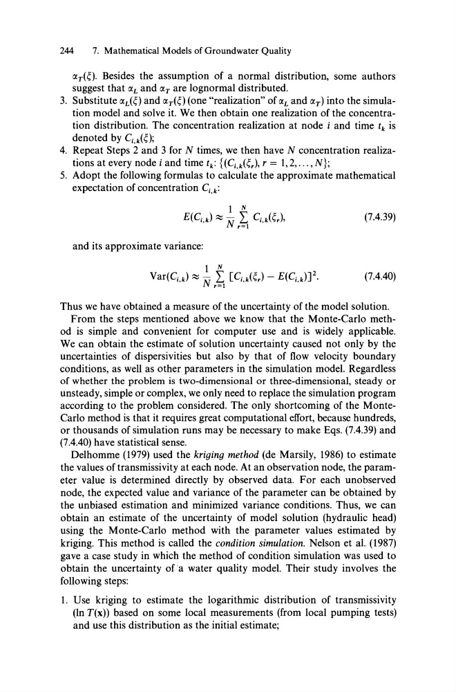
expectation of concentration Ci,k:
(7.4.39)
and its approximate variance:
(7.4.40)
Thus we have obtained a measure of the uncertainty of the model solution.
From the steps mentioned above we know that the Monte-Carlo method is simple and convenient for computer use and is widely applicable.
We can obtain the estimate of solution uncertainty caused not only by the
uncertainties of dispersivities but also by that of flow velocity boundary
conditions, as weIl as other parameters in the simulation model. Regardless
of whether the problem is two-dimensional or three-dimensional, steady or
unsteady, simple or complex, we only need to replace the simulation program
according to the problem considered. The only shortcoming of the MonteCarlo method is that it requires great computational effort, because hundreds,
or thousands of simulation runs may be necessary to make Eqs. (7.4.39) and
(7.4.40) have statistical sense.
Delhomme (1979) used the kriging method (de Marsily, 1986) to estimate
the values of transmissivity at each node. At an observation node, the parameter value is determined directly by observed data. For each unobserved
node, the expected value and variance of the parameter can be obtained by
the unbiased estimation and minimized variance conditions. Thus, we can
obtain an estimate of the uncertainty of model solution (hydraulic head)
using the Monte-Carlo method with the parameter values estimated by
kriging. This method is called the condition simulation. Nelson et al. (1987)
gave a case study in which the method of condition simulation was used to
obtain the uncertainty ofa water quality model. Their study involves the
following steps:
1. Use kriging to estimate the logarithmic distribution of transmissivity
(In T(x)) based on some local measurements (from local pumping tests)
and use this distribution as the initial estimate;
7. Mathematical Models of Groundwater Quality
O(T(e). Besides the assumption of a normal distribution, some authors
suggest that O(L and O(T are lognormal distributed.
3. Substitute O(L(e) and O(T(e) (one "realization" of O(L and O(T) into the simulation model and solve it. We then obtain one realization of the concentration distribution. The concentration realization at node i and time t k is
denoted by Ci,k(e);
4. Repeat Steps 2 and 3 for N times, we then have Neoncentration realizations at every node i and time tk: {(Ci,k(er), r = 1,2, ... , N};
5. Adopt the following formulas to calculate the approximate mathematical
expectation of concentration Ci,k:
(7.4.39)
and its approximate variance:
(7.4.40)
Thus we have obtained a measure of the uncertainty of the model solution.
From the steps mentioned above we know that the Monte-Carlo method is simple and convenient for computer use and is widely applicable.
We can obtain the estimate of solution uncertainty caused not only by the
uncertainties of dispersivities but also by that of flow velocity boundary
conditions, as weIl as other parameters in the simulation model. Regardless
of whether the problem is two-dimensional or three-dimensional, steady or
unsteady, simple or complex, we only need to replace the simulation program
according to the problem considered. The only shortcoming of the MonteCarlo method is that it requires great computational effort, because hundreds,
or thousands of simulation runs may be necessary to make Eqs. (7.4.39) and
(7.4.40) have statistical sense.
Delhomme (1979) used the kriging method (de Marsily, 1986) to estimate
the values of transmissivity at each node. At an observation node, the parameter value is determined directly by observed data. For each unobserved
node, the expected value and variance of the parameter can be obtained by
the unbiased estimation and minimized variance conditions. Thus, we can
obtain an estimate of the uncertainty of model solution (hydraulic head)
using the Monte-Carlo method with the parameter values estimated by
kriging. This method is called the condition simulation. Nelson et al. (1987)
gave a case study in which the method of condition simulation was used to
obtain the uncertainty ofa water quality model. Their study involves the
following steps:
1. Use kriging to estimate the logarithmic distribution of transmissivity
(In T(x)) based on some local measurements (from local pumping tests)
and use this distribution as the initial estimate;