

7.4. Statistic Theory and Uncertainty Analysis
243
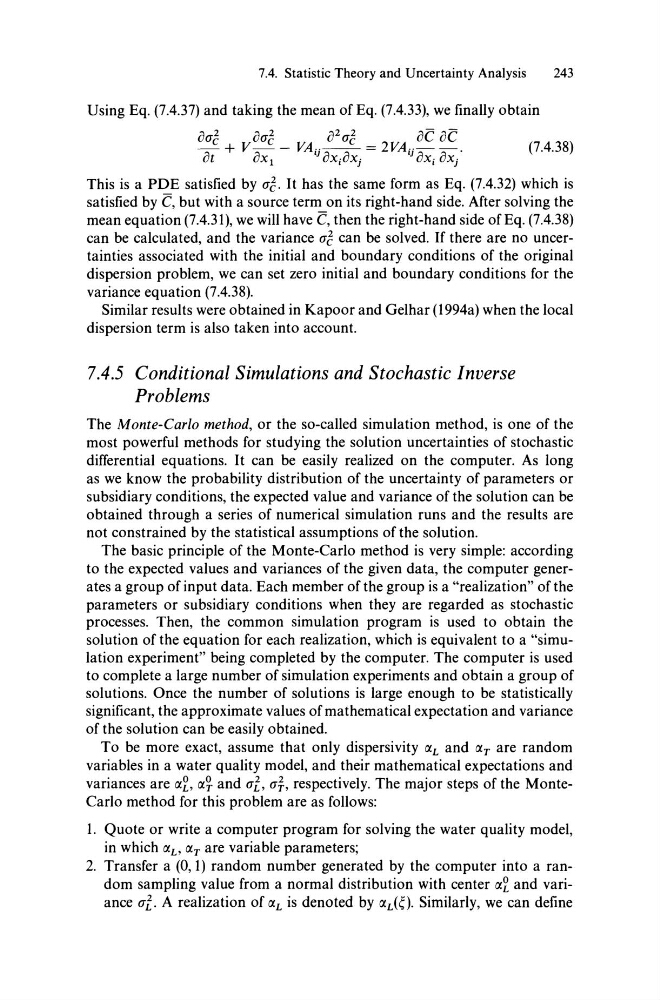
Using Eq. (7.4.37) and taking the mean of Eq. (7.4.33), we finally obtain
o(JE
O(JE
0 2 (JE
oe oe
~ + v ~ - VAij~ = 2VAij~~.
ut
UX I
UXiUXj
uXi UXj
(7.4.38)
This is a PDE satisfied by (JE- It has the same form as Eq. (7.4.32) which is
satisfied by e, but with a source term on its right-hand side. After solving the
mean equation (7.4.31), we will have e, then the right-hand side ofEq. (7.4.38)
can be calculated, and the variance (JE can be solved. If there are no uncertainties associated with the initial and boundary conditions of the original
dispersion problem, we can set zero initial and boundary conditions for the
variance equation (7.4.38).
Similar results were obtained in Kapoor and Gelhar (1994a) when the local
dispersion term is also taken into account.
7.4.5 Conditional Simulations and Stochastic Inverse
Problems
The Monte-Carlo method, or the so-called simulation method, is one of the
most powerful methods for studying the solution uncertainties of stochastic
differential equations. It can be easily realized on the computer. As long
as we know the probability distribution of the uncertainty of parameters or
subsidiary conditions, the expected value and variance of the solution can be
obtained through aseries of numerical simulation runs and the results are
not constrained by the statistical assumptions of the solution.
The basic principle of the Monte-Carlo method is very simple: according
to the expected values and variances of the given data, the computer generates a group ofinput data. Each member ofthe group is a "realization" ofthe
parameters or subsidiary conditions when they are regarded as stochastic
processes. Then, the common simulation program is used to obtain the
solution of the equation for each realization, which is equivalent to a "simulation experiment" being completed by the computer. The computer is used
to complete a large number of simulation experiments and obtain a group of
solutions. Once the number of solutions is large enough to be statistically
significant, the approximate values of mathematical expectation and variance
of the solution can be easily obtained.
To be more exact, ass urne that only dispersivity (XL and (XT are random
variables in a water quality model, and their mathematical expectations and
variances are (X2, (X~ and (Jf., (Ji-, respectively. The major steps of the MonteCarlo method for this problem are as folIows:
1. Quote or write a computer program for solving the water quality model,
in which (XL' (XT are variable parameters;
2. Transfer a (0,1) random number generated by the computer into a random sampling value from a normal distribution with center (X2 and variance (Jf.. A realization oh L is denoted by (XL(~). Similarly, we can define
243
Using Eq. (7.4.37) and taking the mean of Eq. (7.4.33), we finally obtain
o(JE
O(JE
0 2 (JE
oe oe
~ + v ~ - VAij~ = 2VAij~~.
ut
UX I
UXiUXj
uXi UXj
(7.4.38)
This is a PDE satisfied by (JE- It has the same form as Eq. (7.4.32) which is
satisfied by e, but with a source term on its right-hand side. After solving the
mean equation (7.4.31), we will have e, then the right-hand side ofEq. (7.4.38)
can be calculated, and the variance (JE can be solved. If there are no uncertainties associated with the initial and boundary conditions of the original
dispersion problem, we can set zero initial and boundary conditions for the
variance equation (7.4.38).
Similar results were obtained in Kapoor and Gelhar (1994a) when the local
dispersion term is also taken into account.
7.4.5 Conditional Simulations and Stochastic Inverse
Problems
The Monte-Carlo method, or the so-called simulation method, is one of the
most powerful methods for studying the solution uncertainties of stochastic
differential equations. It can be easily realized on the computer. As long
as we know the probability distribution of the uncertainty of parameters or
subsidiary conditions, the expected value and variance of the solution can be
obtained through aseries of numerical simulation runs and the results are
not constrained by the statistical assumptions of the solution.
The basic principle of the Monte-Carlo method is very simple: according
to the expected values and variances of the given data, the computer generates a group ofinput data. Each member ofthe group is a "realization" ofthe
parameters or subsidiary conditions when they are regarded as stochastic
processes. Then, the common simulation program is used to obtain the
solution of the equation for each realization, which is equivalent to a "simulation experiment" being completed by the computer. The computer is used
to complete a large number of simulation experiments and obtain a group of
solutions. Once the number of solutions is large enough to be statistically
significant, the approximate values of mathematical expectation and variance
of the solution can be easily obtained.
To be more exact, ass urne that only dispersivity (XL and (XT are random
variables in a water quality model, and their mathematical expectations and
variances are (X2, (X~ and (Jf., (Ji-, respectively. The major steps of the MonteCarlo method for this problem are as folIows:
1. Quote or write a computer program for solving the water quality model,
in which (XL' (XT are variable parameters;
2. Transfer a (0,1) random number generated by the computer into a random sampling value from a normal distribution with center (X2 and variance (Jf.. A realization oh L is denoted by (XL(~). Similarly, we can define