

238
7. Mathematical Models of Groundwater Quality
ate them with the macrodispersivities Aij defined in Eq. (7.4.9). Note that the
mean equation Eq. (7.4.8) is still an advection-dispersion equation, and Eq.
(7.4.9) is similar to Eq. (7.4.1), but the meaning of dispersion parameters are
changed after upscaling.
Subtracting the mean equation (7.4.8) from Eq. (7.4.5), and only retaining
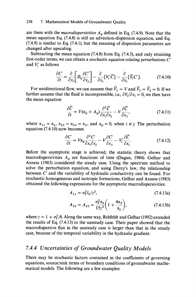
first-order terms, we can obtain a stochastic equation relating perturbations C'
and V;' as follows
0C'
0 [ OC']
0
-
0 -
~ = ~ Dij:;-- - ~[V;'C] - ~[V;C'].
ut
uXi
uXj
uXi
uXi
(7.4.10)
For unidirectional flow, we can ass urne that V 1 = Vand V 2 = V 3 = O.lfwe
further assurne that the fluid is incompressible, i.e., oV;/ox i = 0, we then have
the mean equation
(7.4.11)
where 0(11 = O(u 0(22 = 0(33 = O(T' and O(ij = 0, when i # j. The perturbation
equation (7.4.10) now becomes
0C'
0 2 C'
0C'
oe
- = VO(··--- V - - v,'ot
IJ oxiox j
OX 1
I OX i ·
(7.4.12)
Before the asymptotic stage is achieved, the statistic theory shows that
macrodispersivities Aij are functions of time (Dagan, 1984). Gelhar and
Axness (1983) considered the steady case. Using the spectrum method to
solve the perturbation equation, and using Darcy's law, the relationship
between C' and the variability of hydraulic conductivity can be found. For
stochastic homogeneous and isotropic formations, Gelhar and Axness (1983)
obtained the following expressions for the asymptotic macrodispersivities:
(7.4.13a)
(J~O(L(
40(T)
A 22 = A 33 = 15 y 2 1 + a; ,
(7.4.13b)
where y = 1 + (J~ /6. Along the same way, Rehfeldt and Gelhar (1992) extended
the results of Eq. (7.4.13) to the unsteady case. Their paper showed that the
macrodispersive flux in the unsteady ca se is larger than that in the steady
ca se, because of the temporal variability in the hydraulic gradient.
7.4.4 U ncertainties of Groundwater Quality Models
There may be stochastic factors contained in the coefficients of governing
equations, source/sink terms or boundary conditions of groundwater mathematical models. The following are a few examples:
7. Mathematical Models of Groundwater Quality
ate them with the macrodispersivities Aij defined in Eq. (7.4.9). Note that the
mean equation Eq. (7.4.8) is still an advection-dispersion equation, and Eq.
(7.4.9) is similar to Eq. (7.4.1), but the meaning of dispersion parameters are
changed after upscaling.
Subtracting the mean equation (7.4.8) from Eq. (7.4.5), and only retaining
first-order terms, we can obtain a stochastic equation relating perturbations C'
and V;' as follows
0C'
0 [ OC']
0
-
0 -
~ = ~ Dij:;-- - ~[V;'C] - ~[V;C'].
ut
uXi
uXj
uXi
uXi
(7.4.10)
For unidirectional flow, we can ass urne that V 1 = Vand V 2 = V 3 = O.lfwe
further assurne that the fluid is incompressible, i.e., oV;/ox i = 0, we then have
the mean equation
(7.4.11)
where 0(11 = O(u 0(22 = 0(33 = O(T' and O(ij = 0, when i # j. The perturbation
equation (7.4.10) now becomes
0C'
0 2 C'
0C'
oe
- = VO(··--- V - - v,'ot
IJ oxiox j
OX 1
I OX i ·
(7.4.12)
Before the asymptotic stage is achieved, the statistic theory shows that
macrodispersivities Aij are functions of time (Dagan, 1984). Gelhar and
Axness (1983) considered the steady case. Using the spectrum method to
solve the perturbation equation, and using Darcy's law, the relationship
between C' and the variability of hydraulic conductivity can be found. For
stochastic homogeneous and isotropic formations, Gelhar and Axness (1983)
obtained the following expressions for the asymptotic macrodispersivities:
(7.4.13a)
(J~O(L(
40(T)
A 22 = A 33 = 15 y 2 1 + a; ,
(7.4.13b)
where y = 1 + (J~ /6. Along the same way, Rehfeldt and Gelhar (1992) extended
the results of Eq. (7.4.13) to the unsteady case. Their paper showed that the
macrodispersive flux in the unsteady ca se is larger than that in the steady
ca se, because of the temporal variability in the hydraulic gradient.
7.4.4 U ncertainties of Groundwater Quality Models
There may be stochastic factors contained in the coefficients of governing
equations, source/sink terms or boundary conditions of groundwater mathematical models. The following are a few examples: