

7.4. Statistic Theory and Uncertainty Analysis
237
larger than Iy , the correlation between them is very small. A realization
of a stationary random field can be estimated by kriging when the mean,
covariance function and some point measurements of the field are given. A
complete discussion on geostatistieal methods (kriging and co-kriging) for
estimating stationary and non-stationary random fields can be found in de
Marsily (1986).
In practice, most values of (Ti found in field tests are less than unity,
however, cases of (Ti > 10 are also possible. Values of Iy may change in a
large range, from less than one meter to tens and even hundreds of meters
(Gelhar, 1986).
7.4.3 Stochastic Advectian-Dispersion Equations and
M acrodispersivities
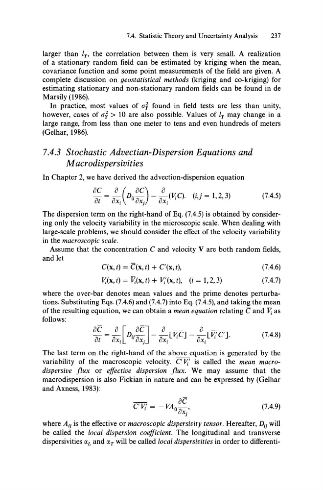
In Chapter 2, we have derived the advection-dispersion equation
OC
0 ( OC)
0
T = ~ Dij~ - ~(ltjC). (i,j = 1,2,3)
ut
uXi
uXj
uXi
(7.4.5)
The dispersion term on the right-hand of Eq. (7.4.5) is obtained by considering only the velocity variability in the microscopic scale. When dealing with
large-scale problems, we should consider the efTect of the velocity variability
in the maeroseopic seale.
Assurne that the concentration C and velocity V are both random fields,
and let
C(x, t) = C(x, t) + C'(x, t),
ltj(x, t) = V;(x, t) + ltj'(x, t), (i = 1,2,3)
(7.4.6)
(7.4.7)
where the over-bar denotes mean values and the prime denotes perturbations. Substituting Eqs. (7.4.6) and (7.4.7) into Eq. (7.4.5), and taking the mean
of the resulting equation, we can obtain a mean equation relating C and V; as
follows:
oC 0 [ OC] 0 - -
i J -
~=~ Dij~ -~[ltjC]-~[ltj'C'].
iJt
iJxi
iJxj
iJxi
OXi
(7.4.8)
The last term on the right-hand of the above equati~n is generated by the
variability of the macroscopic velocity. C' ltj' is called the mean maerodispersive flux or effeetive dispersion flux. We may assurne that the
macrodispersion is also Fickian in nature and can be expressed by (Gelhar
and Axness, 1983):
(7.4.9)
where A ij is the efTective or maeroseopie dispersivity tensor. Hereafter, Dij will
be called the loeal dispersion eoefficient. The longitudinal and transverse
dispersivities (h and (XT will be called loeal dispersivities in order to difTerenti-
237
larger than Iy , the correlation between them is very small. A realization
of a stationary random field can be estimated by kriging when the mean,
covariance function and some point measurements of the field are given. A
complete discussion on geostatistieal methods (kriging and co-kriging) for
estimating stationary and non-stationary random fields can be found in de
Marsily (1986).
In practice, most values of (Ti found in field tests are less than unity,
however, cases of (Ti > 10 are also possible. Values of Iy may change in a
large range, from less than one meter to tens and even hundreds of meters
(Gelhar, 1986).
7.4.3 Stochastic Advectian-Dispersion Equations and
M acrodispersivities
In Chapter 2, we have derived the advection-dispersion equation
OC
0 ( OC)
0
T = ~ Dij~ - ~(ltjC). (i,j = 1,2,3)
ut
uXi
uXj
uXi
(7.4.5)
The dispersion term on the right-hand of Eq. (7.4.5) is obtained by considering only the velocity variability in the microscopic scale. When dealing with
large-scale problems, we should consider the efTect of the velocity variability
in the maeroseopic seale.
Assurne that the concentration C and velocity V are both random fields,
and let
C(x, t) = C(x, t) + C'(x, t),
ltj(x, t) = V;(x, t) + ltj'(x, t), (i = 1,2,3)
(7.4.6)
(7.4.7)
where the over-bar denotes mean values and the prime denotes perturbations. Substituting Eqs. (7.4.6) and (7.4.7) into Eq. (7.4.5), and taking the mean
of the resulting equation, we can obtain a mean equation relating C and V; as
follows:
oC 0 [ OC] 0 - -
i J -
~=~ Dij~ -~[ltjC]-~[ltj'C'].
iJt
iJxi
iJxj
iJxi
OXi
(7.4.8)
The last term on the right-hand of the above equati~n is generated by the
variability of the macroscopic velocity. C' ltj' is called the mean maerodispersive flux or effeetive dispersion flux. We may assurne that the
macrodispersion is also Fickian in nature and can be expressed by (Gelhar
and Axness, 1983):
(7.4.9)
where A ij is the efTective or maeroseopie dispersivity tensor. Hereafter, Dij will
be called the loeal dispersion eoefficient. The longitudinal and transverse
dispersivities (h and (XT will be called loeal dispersivities in order to difTerenti-