

7.2. Model Calibration and Parameter Estimation
221
c
o
4
8
12
16
20 t(d)
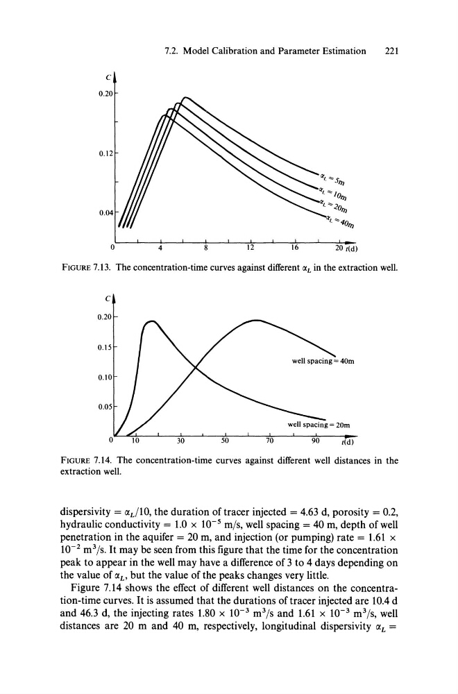
FIGURE 7.13. The concentration-time curves against different !XL in the extraction well.
c
FIGURE 7.14. The concentration-time curves against different well distances in the
extraction weil.
dispersivity = (Xdl0, the duration of tracer injected = 4.63 d, porosity = 0.2,
hydraulic conductivity = 1.0 x 10⁻⁵ m/s, weH spacing = 40 m, depth of weH
penetration in the aquifer = 20 m, and injection (or pumping) rate = 1.61 x
10- 2 m 3 /s.1t may be seen from this figure that the time for the concentration
peak to appear in the weH may have a difference of 3 to 4 days depending on
the value of (XL> but the value of the peaks changes very little.
Figure 7.14 shows the effect of different weH distances on the concentration-time curves. It is assumed that the durations of tracer injected are 10.4 d
and 46.3 d, the injecting rates 1.80 x 10- 3 m 3 /s and 1.61 x 10- 3 m 3 /s, weH
distances are 20 m and 40 m, respectively, longitudinal dispersivity (XL =
221
c
o
4
8
12
16
20 t(d)
FIGURE 7.13. The concentration-time curves against different !XL in the extraction well.
c
FIGURE 7.14. The concentration-time curves against different well distances in the
extraction weil.
dispersivity = (Xdl0, the duration of tracer injected = 4.63 d, porosity = 0.2,
hydraulic conductivity = 1.0 x 10⁻⁵ m/s, weH spacing = 40 m, depth of weH
penetration in the aquifer = 20 m, and injection (or pumping) rate = 1.61 x
10- 2 m 3 /s.1t may be seen from this figure that the time for the concentration
peak to appear in the weH may have a difference of 3 to 4 days depending on
the value of (XL> but the value of the peaks changes very little.
Figure 7.14 shows the effect of different weH distances on the concentration-time curves. It is assumed that the durations of tracer injected are 10.4 d
and 46.3 d, the injecting rates 1.80 x 10- 3 m 3 /s and 1.61 x 10- 3 m 3 /s, weH
distances are 20 m and 40 m, respectively, longitudinal dispersivity (XL =