

7.2. Model Calibration and Parameter Estimation
205
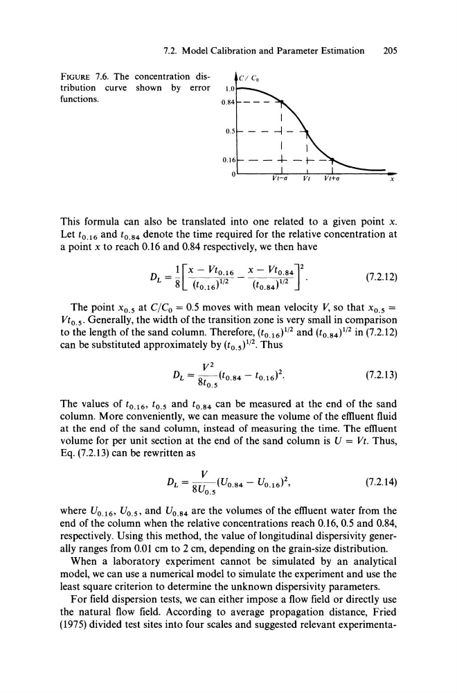
FIGURE 7.6. The concentration disCI Co
tribution curve shown by error
functions.
x
This formula can also be translated into one related to a given point x.
Let t O . 16 and t O . 84 denote the time required for the relative concentration at
a point x to reach 0.16 and 0.84 respectively, we then have
_ 1 [x - VtO .16 x - VtO .84J2
D L - 8" (t )1/2 - (t )1/2
0.16
0.84
(7.2.12)
The point X o . s at C/C o = 0.5 moves with mean velocity V, so that x o . s =
Vt o . s . Generally, the width of the transition zone is very small in comparison
to the length of the sand column. Therefore, (t O • 16 )1/2 and (t O . 84 )1/2 in (7.2.12)
can be substituted approximately by (t0.S)1/2. Thus
V 2
DL = ~(tO.84 - t O. 16 )2.
0.5
(7.2.13)
The values of tO.16' to.s and tO•84 can be measured at the end of the sand
column. More conveniently, we can measure the volume of the emuent fluid
at the end of the sand column, instead of measuring the time. The emuent
volume for per unit section at the end of the sand column is U = Vt. Thus,
Eq. (7.2.13) can be rewritten as
(7.2.14)
where UO.16 ' UO.5 , and UO.84 are the volumes of the emuent water from the
end of the column when the relative concentrations reach 0.16, 0.5 and 0.84,
respectively. Using this method, the value of longitudinal dispersivity generally ranges from 0.01 cm to 2 cm, depending on the grain-size distribution.
When a laboratory experiment cannot be simulated by an analytical
model, we can use a numerical model to simulate the experiment and use the
least square criterion to determine the unknown dispersivity parameters.
For field dispersion tests, we can either impose a flow field or directly use
the natural flow field. According to average propagation distance, Fried
(1975) divided test sites into four scales and suggested relevant experimenta-
205
FIGURE 7.6. The concentration disCI Co
tribution curve shown by error
functions.
x
This formula can also be translated into one related to a given point x.
Let t O . 16 and t O . 84 denote the time required for the relative concentration at
a point x to reach 0.16 and 0.84 respectively, we then have
_ 1 [x - VtO .16 x - VtO .84J2
D L - 8" (t )1/2 - (t )1/2
0.16
0.84
(7.2.12)
The point X o . s at C/C o = 0.5 moves with mean velocity V, so that x o . s =
Vt o . s . Generally, the width of the transition zone is very small in comparison
to the length of the sand column. Therefore, (t O • 16 )1/2 and (t O . 84 )1/2 in (7.2.12)
can be substituted approximately by (t0.S)1/2. Thus
V 2
DL = ~(tO.84 - t O. 16 )2.
0.5
(7.2.13)
The values of tO.16' to.s and tO•84 can be measured at the end of the sand
column. More conveniently, we can measure the volume of the emuent fluid
at the end of the sand column, instead of measuring the time. The emuent
volume for per unit section at the end of the sand column is U = Vt. Thus,
Eq. (7.2.13) can be rewritten as
(7.2.14)
where UO.16 ' UO.5 , and UO.84 are the volumes of the emuent water from the
end of the column when the relative concentrations reach 0.16, 0.5 and 0.84,
respectively. Using this method, the value of longitudinal dispersivity generally ranges from 0.01 cm to 2 cm, depending on the grain-size distribution.
When a laboratory experiment cannot be simulated by an analytical
model, we can use a numerical model to simulate the experiment and use the
least square criterion to determine the unknown dispersivity parameters.
For field dispersion tests, we can either impose a flow field or directly use
the natural flow field. According to average propagation distance, Fried
(1975) divided test sites into four scales and suggested relevant experimenta-