

7.1. The Classification ofGroundwater Quality Models
197
conditions are still required. In practice, it is very difficult to obtain all of
these data.
If we only concern the average level of pollution in an aquifer and want to
predict its variation with time, the so-called "black-box model" or a single
element model can be used. In this kind of model, the concentration only
depends on time, not on space. Therefore, it is often called the lumped parameter model of water quality.
Let us imagine an aquifer as a black-box where pollutants flow in or out.
By analyzing the observed input-output data, we may find an input-output
relationship of the box, although the structure of the box is unknown. Once
the input-output relationship is found, we can use it to predict the aquifer
response (model output) corresponding to any excitation to the aquifer. For
instance, rainfall may bring contaminants from the ground surface into the
aquifer (input) and then drains them into a river (output). If we only wish to
know the relationship between input and output, rather than the pollution
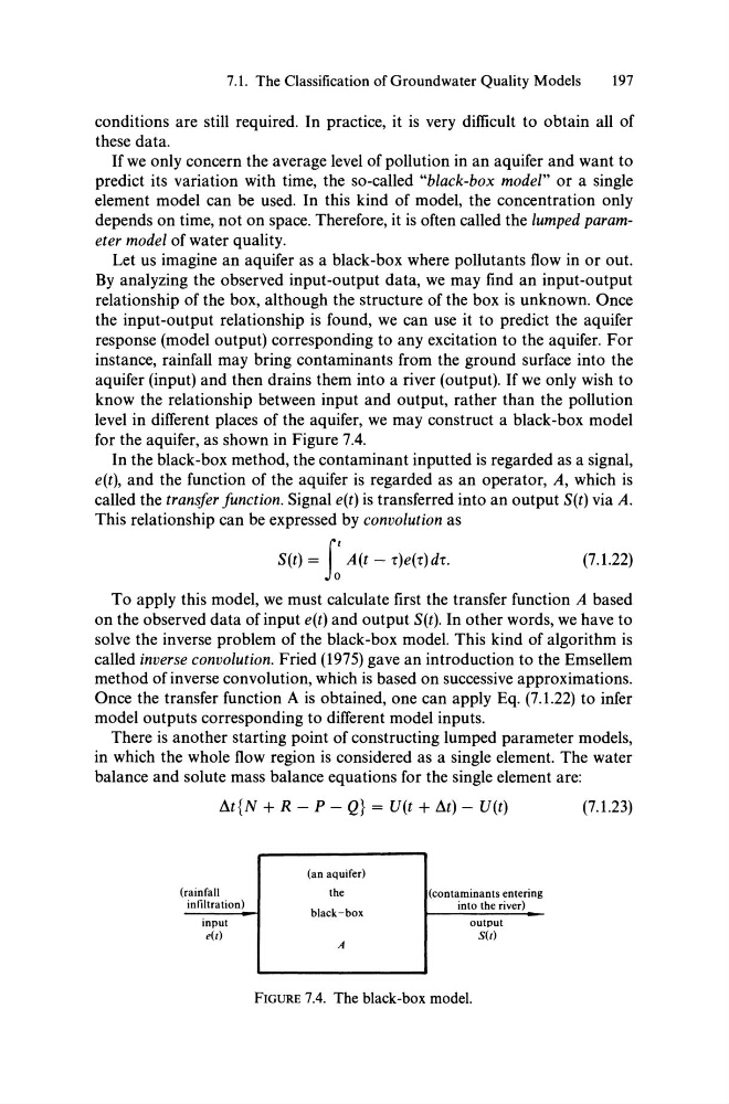
level in different places of the aquifer, we may construct a black-box model
for the aquifer, as shown in Figure 7.4.
In the black-box method, the contaminant inputted is regarded as a signal,
e(t), and the function of the aquifer is regarded as an operator, A, which is
called the transfer function. Signal e(t) is transferred into an output S(t) via A.
This relationship can be expressed by convolution as
S(t) = I A(t - t)e(t)dt.
(7.1.22)
To apply this model, we must calculate first the transfer function A based
on the observed data of input e(t) and output S(t). In other words, we have to
solve the inverse problem of the black-box model. This kind of algorithm is
called inverse convolution. Fried (1975) gave an introduction to the Emsellem
method ofinverse convolution, which is based on successive approximations.
Once the transfer function A is obtained, one can apply Eq. (7.1.22) to infer
model outputs corresponding to different model inputs.
There is another starting point of constructing lumped parameter models,
in which the whole flow region is considered as a single element. The water
balance and solute mass balance equations for the single element are:
~t{N + R - P - Q} = U(t + ~t) - U(t)
(rainfall
infiltration)
input
e(t}
(an aquifer)
the
black-box
A
(contaminants entering
into the river)
output
S(t}
FIGURE 7.4. The black-box model.
(7.1.23)
197
conditions are still required. In practice, it is very difficult to obtain all of
these data.
If we only concern the average level of pollution in an aquifer and want to
predict its variation with time, the so-called "black-box model" or a single
element model can be used. In this kind of model, the concentration only
depends on time, not on space. Therefore, it is often called the lumped parameter model of water quality.
Let us imagine an aquifer as a black-box where pollutants flow in or out.
By analyzing the observed input-output data, we may find an input-output
relationship of the box, although the structure of the box is unknown. Once
the input-output relationship is found, we can use it to predict the aquifer
response (model output) corresponding to any excitation to the aquifer. For
instance, rainfall may bring contaminants from the ground surface into the
aquifer (input) and then drains them into a river (output). If we only wish to
know the relationship between input and output, rather than the pollution
level in different places of the aquifer, we may construct a black-box model
for the aquifer, as shown in Figure 7.4.
In the black-box method, the contaminant inputted is regarded as a signal,
e(t), and the function of the aquifer is regarded as an operator, A, which is
called the transfer function. Signal e(t) is transferred into an output S(t) via A.
This relationship can be expressed by convolution as
S(t) = I A(t - t)e(t)dt.
(7.1.22)
To apply this model, we must calculate first the transfer function A based
on the observed data of input e(t) and output S(t). In other words, we have to
solve the inverse problem of the black-box model. This kind of algorithm is
called inverse convolution. Fried (1975) gave an introduction to the Emsellem
method ofinverse convolution, which is based on successive approximations.
Once the transfer function A is obtained, one can apply Eq. (7.1.22) to infer
model outputs corresponding to different model inputs.
There is another starting point of constructing lumped parameter models,
in which the whole flow region is considered as a single element. The water
balance and solute mass balance equations for the single element are:
~t{N + R - P - Q} = U(t + ~t) - U(t)
(rainfall
infiltration)
input
e(t}
(an aquifer)
the
black-box
A
(contaminants entering
into the river)
output
S(t}
FIGURE 7.4. The black-box model.
(7.1.23)