

6.4. The Modified Methods of Characteristics
179
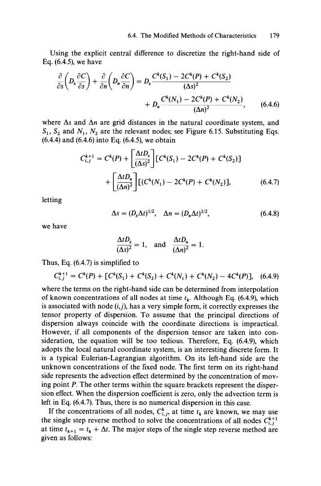
Using the explicit central difTerence to discretize the right-hand side of
Eq. (6.4.5), we have
o ( OC) 0 ( OC) _ Ck(Sl) - 2C k (P) + Ck(Sz)
os D s as + on D n on - D s
(~s)z
Ck(N l ) - 2C k (P) + Ck(N z )
+ D n
(~nf
'
(6.4.6)
where ~s and ~n are grid distances in the natural coordinate system, and
Sl' Sz and Nb Nz are the relevant no des; see Figure 6.15. Substituting Eqs.
(6.4.4) and (6.4.6) into Eq. (6.4.5), we obtain
letting
we have
ct? = Ck(P) + [~~~ ] [Ck(Sd - 2C k (P) + Ck(Sz)]
[ ~tDnJ k
k
k
+ (~n)Z [(C (Nl ) - 2C (P) + C (Nz )],
MD s = 1 and ~tDn = 1
(~s)Z'
(~n)z'
Thus, Eq. (6.4.7) is simplified to
(6.4.7)
(6.4.8)
ct1 l = Ck(P) + [Ck(Sl) + Ck(Sz) + Ck(Nd + Ck(N z ) - 4C k (P)], (6.4.9)
where the terms on the right-hand side can be determined from interpolation
of known concentrations of all nodes at time t k • Although Eq. (6.4.9), which
is associated with node (i,j), has a very simple form, it correctly expresses the
tensor property of dispersion. To assume that the principal directions of
dispersion always coincide with the coordinate directions is impractical.
However, if all components of the dispersion tensor are taken into consideration, the equation will be too tedious. Therefore, Eq. (6.4.9), which
adopts the local natural co ordinate system, is an interesting discrete form. It
is a typical Eulerian-Lagrangian algorithm. On its left-hand side are the
unknown concentrations of the fixed node. The first term on its right-hand
side represents the advection efTect determined by the concentration of moving point P. The other terms within the square brackets represent the dispersion efTect. When the dispersion coefficient is zero, only the advection term is
left in Eq. (6.4.7). Thus, there is no numerical dispersion in this case.
If the concentrations of all nodes, CL, at time t k are known, we may use
the single step reverse method to solve the concentrations of all nodes ct1 l
at time tk+l = tk + ~t. The major steps of the single step reverse method are
given as follows:
179
Using the explicit central difTerence to discretize the right-hand side of
Eq. (6.4.5), we have
o ( OC) 0 ( OC) _ Ck(Sl) - 2C k (P) + Ck(Sz)
os D s as + on D n on - D s
(~s)z
Ck(N l ) - 2C k (P) + Ck(N z )
+ D n
(~nf
'
(6.4.6)
where ~s and ~n are grid distances in the natural coordinate system, and
Sl' Sz and Nb Nz are the relevant no des; see Figure 6.15. Substituting Eqs.
(6.4.4) and (6.4.6) into Eq. (6.4.5), we obtain
letting
we have
ct? = Ck(P) + [~~~ ] [Ck(Sd - 2C k (P) + Ck(Sz)]
[ ~tDnJ k
k
k
+ (~n)Z [(C (Nl ) - 2C (P) + C (Nz )],
MD s = 1 and ~tDn = 1
(~s)Z'
(~n)z'
Thus, Eq. (6.4.7) is simplified to
(6.4.7)
(6.4.8)
ct1 l = Ck(P) + [Ck(Sl) + Ck(Sz) + Ck(Nd + Ck(N z ) - 4C k (P)], (6.4.9)
where the terms on the right-hand side can be determined from interpolation
of known concentrations of all nodes at time t k • Although Eq. (6.4.9), which
is associated with node (i,j), has a very simple form, it correctly expresses the
tensor property of dispersion. To assume that the principal directions of
dispersion always coincide with the coordinate directions is impractical.
However, if all components of the dispersion tensor are taken into consideration, the equation will be too tedious. Therefore, Eq. (6.4.9), which
adopts the local natural co ordinate system, is an interesting discrete form. It
is a typical Eulerian-Lagrangian algorithm. On its left-hand side are the
unknown concentrations of the fixed node. The first term on its right-hand
side represents the advection efTect determined by the concentration of moving point P. The other terms within the square brackets represent the dispersion efTect. When the dispersion coefficient is zero, only the advection term is
left in Eq. (6.4.7). Thus, there is no numerical dispersion in this case.
If the concentrations of all nodes, CL, at time t k are known, we may use
the single step reverse method to solve the concentrations of all nodes ct1 l
at time tk+l = tk + ~t. The major steps of the single step reverse method are
given as follows: