

178
6. Numerical Solutions of Advection-Dominated Problems
•
•
N-.... -....
/s
I
•
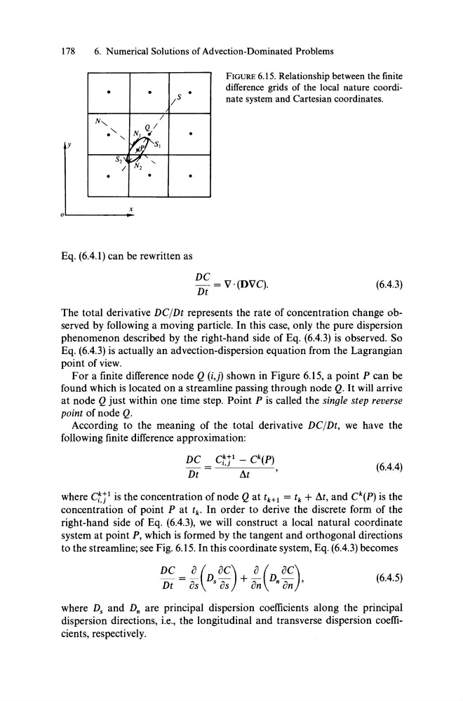
FIGURE 6.15. Relationship between the finite
difference grids of the Iocal nature coordinate system and Cartesian coordinates.
y
NI Q./
•
· "- 1;:[SI
S2~
r.:, "I
•
•
·
x
oL..-------1~
Eq. (6.4.1) can be rewritten as
DC = V. (DVC).
Dt
(6.4.3)
The total derivative DC/Dt represents the rate of concentration change observed by following a moving particle. In this case, only the pure dispersion
phenomenon described by the right-hand side of Eq. (6.4.3) is observed. So
Eq. (6.4.3) is actually an advection-dispersion equation from the Lagrangian
point of view.
For a finite difference node Q (i,j) shown in Figure 6.15, a point P can be
found which is located on a streamline passing through node Q. It will arrive
at node Q just within one time step. Point P is called the single step reverse
point of node Q.
According to the meaning of the total derivative DC/Dt, we have the
following finite difference approximation:
(6.4.4)
where ctt 1 is the concentration of node Q at tk+l = t k + M, and Ck(P) is the
concentration of point P at t k • In order to derive the discrete form of the
right-hand side of Eq. (6.4.3), we will construct a local natural coordinate
system at point P, which is formed by the tangent and orthogonal directions
to the streamline; see Fig. 6.15. In this coordinate system, Eq. (6.4.3) becomes
DC
0 ( OC) 0 ( OC)
Dt = os D. es + on D n on '
(6.4.5)
where D. and D n are principal dispersion coefficients along the principal
dispersion directions, i.e., the longitudinal and transverse dispersion coefficients, respectively.
6. Numerical Solutions of Advection-Dominated Problems
•
•
N-.... -....
/s
I
•
FIGURE 6.15. Relationship between the finite
difference grids of the Iocal nature coordinate system and Cartesian coordinates.
y
NI Q./
•
· "- 1;:[SI
S2~
r.:, "I
•
•
·
x
oL..-------1~
Eq. (6.4.1) can be rewritten as
DC = V. (DVC).
Dt
(6.4.3)
The total derivative DC/Dt represents the rate of concentration change observed by following a moving particle. In this case, only the pure dispersion
phenomenon described by the right-hand side of Eq. (6.4.3) is observed. So
Eq. (6.4.3) is actually an advection-dispersion equation from the Lagrangian
point of view.
For a finite difference node Q (i,j) shown in Figure 6.15, a point P can be
found which is located on a streamline passing through node Q. It will arrive
at node Q just within one time step. Point P is called the single step reverse
point of node Q.
According to the meaning of the total derivative DC/Dt, we have the
following finite difference approximation:
(6.4.4)
where ctt 1 is the concentration of node Q at tk+l = t k + M, and Ck(P) is the
concentration of point P at t k • In order to derive the discrete form of the
right-hand side of Eq. (6.4.3), we will construct a local natural coordinate
system at point P, which is formed by the tangent and orthogonal directions
to the streamline; see Fig. 6.15. In this coordinate system, Eq. (6.4.3) becomes
DC
0 ( OC) 0 ( OC)
Dt = os D. es + on D n on '
(6.4.5)
where D. and D n are principal dispersion coefficients along the principal
dispersion directions, i.e., the longitudinal and transverse dispersion coefficients, respectively.