

174
c
6. Numerical Solutions of Advection-Dominated Problems
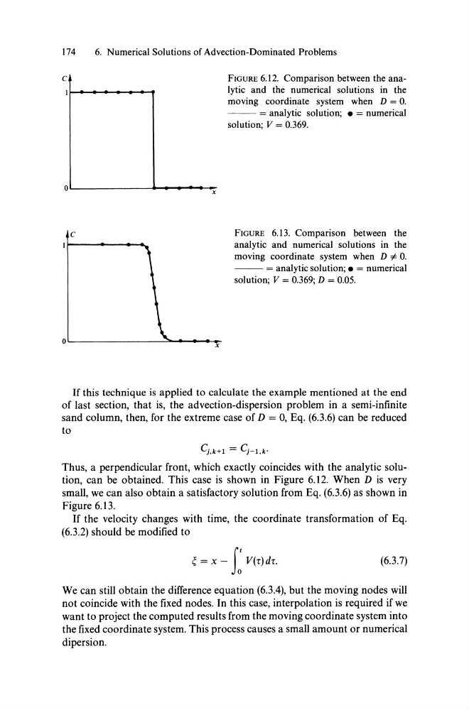
FIGURE 6.12. Comparison between the analytic and the numerical solutions in the
moving coordinate system when D = O.
- - = analytic solution; • = numerical
solution; V = 0.369.
OL-------------~.-.-~~~x
c
FIGURE 6.13. Comparison between the
analytic and numerical solutions in the
moving coordinate system when D". O.
- - = analytic solution; • = numerical
solution; V = 0.369; D = 0.05.
OL---------------~~~~~x
If this technique is applied to calculate the example mentioned at the end
of last section, that is, the advection-dispersion problem in a semi-infinite
sand column, then, for the extreme case of D = 0, Eq. (6.3.6) can be reduced
to
Cj,k+l = Cj-l,k'
Thus, a perpendicular front, which exactly coincides with the analytic solution, can be obtained. This case is shown in Figure 6.12. When D is very
smalI, we can also obtain a satisfactory solution from Eq. (6.3.6) as shown in
Figure 6.13.
If the velocity changes with time, the coordinate transformation of Eq.
(6.3.2) should be modified to
~ = x - t V(r)dr.
(6.3.7)
We can still obtain the difference equation (6.3.4), but the moving nodes will
not coincide with the fixed nodes. In this case, interpolation is required if we
want to project the computed results from the moving co ordinate system into
the fixed co ordinate system. This process causes a small amount or numerical
dipersion.
c
6. Numerical Solutions of Advection-Dominated Problems
FIGURE 6.12. Comparison between the analytic and the numerical solutions in the
moving coordinate system when D = O.
- - = analytic solution; • = numerical
solution; V = 0.369.
OL-------------~.-.-~~~x
c
FIGURE 6.13. Comparison between the
analytic and numerical solutions in the
moving coordinate system when D". O.
- - = analytic solution; • = numerical
solution; V = 0.369; D = 0.05.
OL---------------~~~~~x
If this technique is applied to calculate the example mentioned at the end
of last section, that is, the advection-dispersion problem in a semi-infinite
sand column, then, for the extreme case of D = 0, Eq. (6.3.6) can be reduced
to
Cj,k+l = Cj-l,k'
Thus, a perpendicular front, which exactly coincides with the analytic solution, can be obtained. This case is shown in Figure 6.12. When D is very
smalI, we can also obtain a satisfactory solution from Eq. (6.3.6) as shown in
Figure 6.13.
If the velocity changes with time, the coordinate transformation of Eq.
(6.3.2) should be modified to
~ = x - t V(r)dr.
(6.3.7)
We can still obtain the difference equation (6.3.4), but the moving nodes will
not coincide with the fixed nodes. In this case, interpolation is required if we
want to project the computed results from the moving co ordinate system into
the fixed co ordinate system. This process causes a small amount or numerical
dipersion.