

6.3. Moving Coordinate System and Moving Point Methods
173
nate transformation
e = x - Vt,
Eq. (6.3.1) can be transformed into
ac*
a 2 c*
Tt- D ae2 =0,
(6.3.2)
(6.3.3)
where C*(e, t) is the concentration observed in the moving coordinate system.
Since there is no advection term in Eq. (6.3.3), any numerical scheme can be
used to solve it without numerical difficulty. For instance, we can use the
explicit difference method to obtain
q:k+l - C;'~k _ D Ci\l.k - 2Ctk + Cf-l,k = 0
Al
(.1e)2
'
(6.3.4)
where C;'':k and Ctk+1 are concentrations of node i in the moving coordinate
system at time tk and tk+l = tk + .1t, respectively, while Ct-l,k and Ci"+l,k are
concentrations of nodes i - 1 and i + 1 in the system at time t k •
If the spatial step is taken as .1e = V.1t, then from Eq. (6.3.4), we have:
Ctk+l = Ctk + D(Ct-l,k - 2Ctk + Ci"+1,k)/V 2 Al.
(6.3.5)
The concentrations of all nodes in the system can be solved using the explicit
scheme. This is the solution associated with the moving coordinate system.
Customarily, we wish to obtain the spatial distribution of the concentration
at any assigned time. Thus we have to transform, or project, the results
obtained from the moving co ordinate system into a fixed coordinate system.
For the simplest case being discussed now, we may take x = VAl as the
spatial distance, i.e., take the Courant number VAl/.1x = 1. Consequently,
the nodes in the moving coordinate system always coincide with those in the
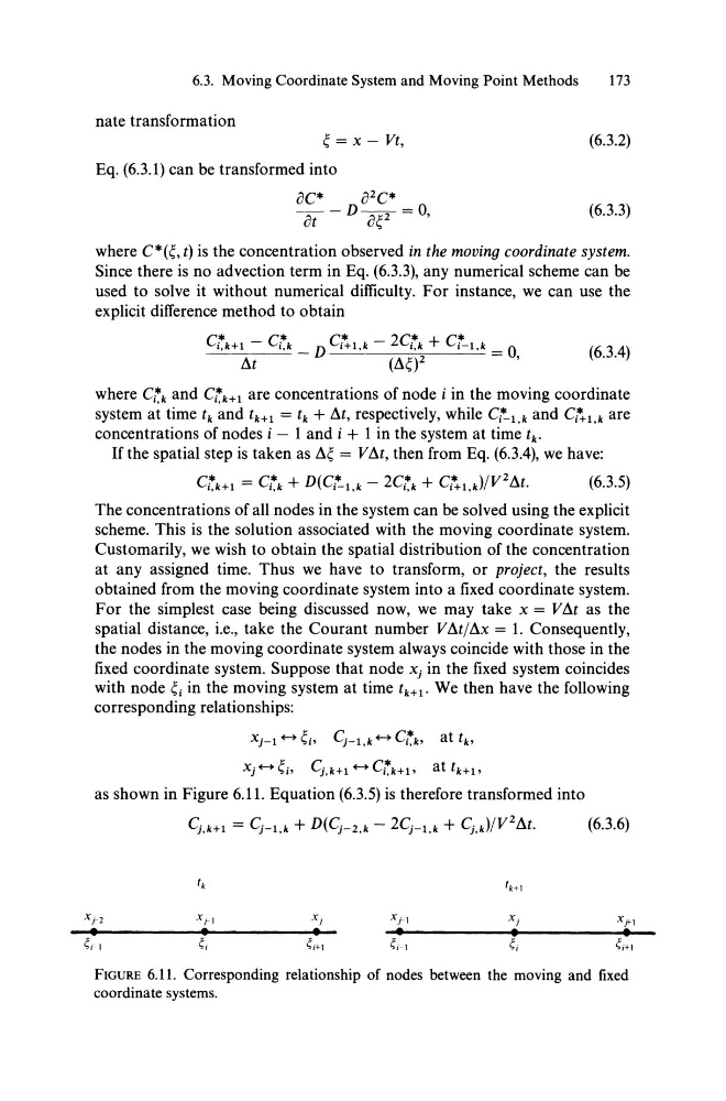
fixed co ordinate system. Suppose that node xj in the fixed system coincides
with node ei in the moving system at time tk+l' We then have the following
corresponding relationships:
Xj - l +-+ ei' Cj-l,k +-+ Ctk' at tk,
Xj +-+ ei' Cj,k+l +-+ Ctk+l' at tk +l ,
as shown in Figure 6.11. Equation (6.3.5) is therefore transformed into
f k
f k+1
Xj-2
Xj-l
X j
Xj-l
X j
•
•
•
•
•
~i 1
~i
~i+l
~H
~i
(6.3.6)
Xfrl
•
~i+l
FIGURE 6.11. Corresponding relationship of nodes between the moving and fixed
coordinate systems.
173
nate transformation
e = x - Vt,
Eq. (6.3.1) can be transformed into
ac*
a 2 c*
Tt- D ae2 =0,
(6.3.2)
(6.3.3)
where C*(e, t) is the concentration observed in the moving coordinate system.
Since there is no advection term in Eq. (6.3.3), any numerical scheme can be
used to solve it without numerical difficulty. For instance, we can use the
explicit difference method to obtain
q:k+l - C;'~k _ D Ci\l.k - 2Ctk + Cf-l,k = 0
Al
(.1e)2
'
(6.3.4)
where C;'':k and Ctk+1 are concentrations of node i in the moving coordinate
system at time tk and tk+l = tk + .1t, respectively, while Ct-l,k and Ci"+l,k are
concentrations of nodes i - 1 and i + 1 in the system at time t k •
If the spatial step is taken as .1e = V.1t, then from Eq. (6.3.4), we have:
Ctk+l = Ctk + D(Ct-l,k - 2Ctk + Ci"+1,k)/V 2 Al.
(6.3.5)
The concentrations of all nodes in the system can be solved using the explicit
scheme. This is the solution associated with the moving coordinate system.
Customarily, we wish to obtain the spatial distribution of the concentration
at any assigned time. Thus we have to transform, or project, the results
obtained from the moving co ordinate system into a fixed coordinate system.
For the simplest case being discussed now, we may take x = VAl as the
spatial distance, i.e., take the Courant number VAl/.1x = 1. Consequently,
the nodes in the moving coordinate system always coincide with those in the
fixed co ordinate system. Suppose that node xj in the fixed system coincides
with node ei in the moving system at time tk+l' We then have the following
corresponding relationships:
Xj - l +-+ ei' Cj-l,k +-+ Ctk' at tk,
Xj +-+ ei' Cj,k+l +-+ Ctk+l' at tk +l ,
as shown in Figure 6.11. Equation (6.3.5) is therefore transformed into
f k
f k+1
Xj-2
Xj-l
X j
Xj-l
X j
•
•
•
•
•
~i 1
~i
~i+l
~H
~i
(6.3.6)
Xfrl
•
~i+l
FIGURE 6.11. Corresponding relationship of nodes between the moving and fixed
coordinate systems.