

170
6. Numerical Solutions of Advection-Dominated Problems
and l';j, Jo}k' v"i are the projections of Von ij,Jk and ki, respectively. Let
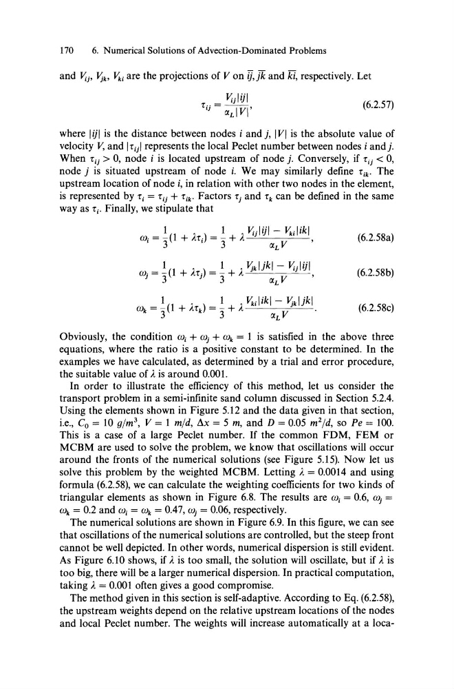
(6.2.57)
where I ijI is the distance between nodes i and j, IVI is the absolute value of
velocity V, and ILUI represents the local PecIet number between nodes i andj.
When Lij > 0, node i is located upstream of node j. Conversely, if Li} < 0,
node j is situated upstream of node i. We may similarly define Lik. The
upstream location of node i, in relation with other two nodes in the element,
is represented by Li = Lij + Lik. Factors Lj and Lk can be defined in the same
way as Li. FinaIly, we stipulate that
(6.2.58a)
(6.2.58b)
(6.2.58c)
Obviously, the condition wi + wj + Wr.: = 1 is satisfied in the above three
equations, where the ratio is a positive constant to be determined. In the
examples we have caIculated, as determined by a trial and error procedure,
the suitable value of A is around 0.001.
In order to illustrate the efficiency of this method, let us consider the
transport problem in a semi-infinite sand column discussed in Section 5.2.4.
Using the elements shown in Figure 5.12 and the data given in that section,
i.e., Co = 10 glm 3 , V = 1 mld, L\x = 5 m, and D = 0.05 m 2 ld, so Pe == 100.
This is a case of a large PecIet number. If the common FDM, FEM or
MCBM are used to solve the problem, we know that oscillations will occur
around the fronts of the numerical solutions (see Figure 5.15). Now let us
solve this problem by the weighted MCBM. Letting A = 0.0014 and using
formula (6.2.58), we can caIculate the weighting coefficients for two kinds of
triangular elements as shown in Figure 6.8. The results are W i = 0.6, wj =
Wr.: = 0.2 and W i = Wr.: = 0.47, Wj = 0.06, respectively.
The numerical solutions are shown in Figure 6.9. In this figure, we can see
that oscillations of the numerical solutions are controIled, but the steep front
cannot be weIl depicted. In other words, numerical dispersion is still evident.
As Figure 6.10 shows, if Ais too smaIl, the solution will oscillate, but if Ais
too big, there will be a larger numerical dispersion. In practical computation,
taking A = 0.001 often gives a good compromise.
The method given in this section is self-adaptive. According to Eq. (6.2.58),
the upstream weights depend on the relative upstream locations of the nodes
and local PecIet number. The weights will increase automatically at a loca-
6. Numerical Solutions of Advection-Dominated Problems
and l';j, Jo}k' v"i are the projections of Von ij,Jk and ki, respectively. Let
(6.2.57)
where I ijI is the distance between nodes i and j, IVI is the absolute value of
velocity V, and ILUI represents the local PecIet number between nodes i andj.
When Lij > 0, node i is located upstream of node j. Conversely, if Li} < 0,
node j is situated upstream of node i. We may similarly define Lik. The
upstream location of node i, in relation with other two nodes in the element,
is represented by Li = Lij + Lik. Factors Lj and Lk can be defined in the same
way as Li. FinaIly, we stipulate that
(6.2.58a)
(6.2.58b)
(6.2.58c)
Obviously, the condition wi + wj + Wr.: = 1 is satisfied in the above three
equations, where the ratio is a positive constant to be determined. In the
examples we have caIculated, as determined by a trial and error procedure,
the suitable value of A is around 0.001.
In order to illustrate the efficiency of this method, let us consider the
transport problem in a semi-infinite sand column discussed in Section 5.2.4.
Using the elements shown in Figure 5.12 and the data given in that section,
i.e., Co = 10 glm 3 , V = 1 mld, L\x = 5 m, and D = 0.05 m 2 ld, so Pe == 100.
This is a case of a large PecIet number. If the common FDM, FEM or
MCBM are used to solve the problem, we know that oscillations will occur
around the fronts of the numerical solutions (see Figure 5.15). Now let us
solve this problem by the weighted MCBM. Letting A = 0.0014 and using
formula (6.2.58), we can caIculate the weighting coefficients for two kinds of
triangular elements as shown in Figure 6.8. The results are W i = 0.6, wj =
Wr.: = 0.2 and W i = Wr.: = 0.47, Wj = 0.06, respectively.
The numerical solutions are shown in Figure 6.9. In this figure, we can see
that oscillations of the numerical solutions are controIled, but the steep front
cannot be weIl depicted. In other words, numerical dispersion is still evident.
As Figure 6.10 shows, if Ais too smaIl, the solution will oscillate, but if Ais
too big, there will be a larger numerical dispersion. In practical computation,
taking A = 0.001 often gives a good compromise.
The method given in this section is self-adaptive. According to Eq. (6.2.58),
the upstream weights depend on the relative upstream locations of the nodes
and local PecIet number. The weights will increase automatically at a loca-