

6.2. Upstream Weighted Methods
169
where
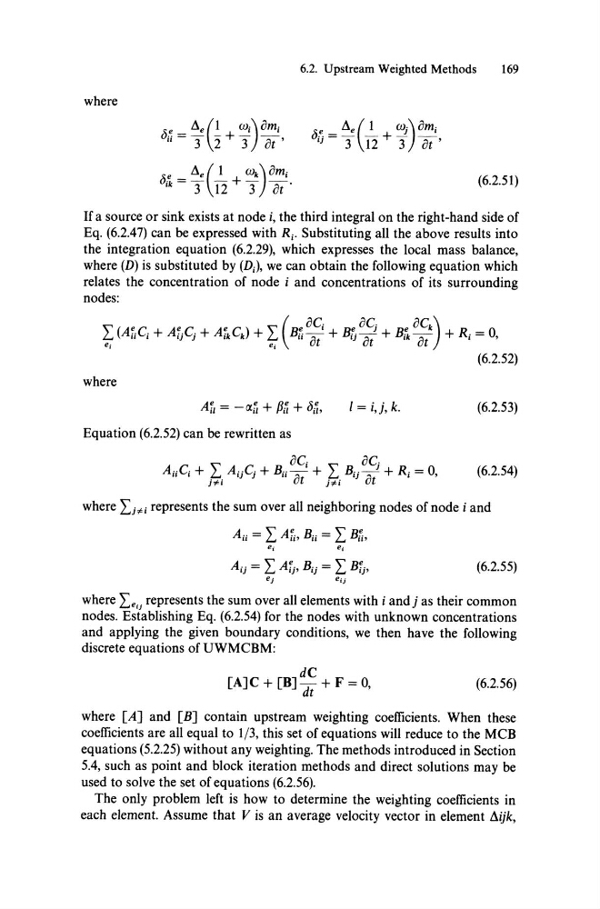
(j.~ = Ae (! W i ) omi
11
3 2 + 3 ot'
(6.2.51)
If a source or sink exists at node i, the third integral on the right-hand side of
Eq. (6.2.47) can be expressed with R i . Substituting all the above results into
the integration equation (6.2.29), which expresses the local mass balance,
where (D) is substituted by (Di ), we can obtain the following equation wh ich
relates the concentration of node i and concentrations of its surrounding
nodes:
"( e C
e C
e C ) " (Be oC i Be oC j Be OCk) R - 0
I... A ii i+Aij j+Aik k +1... ii~+ ij~+ ik~ + i - ,
ei
ei
ut
ut
ut
(6.2.52)
where
1= i,j, k.
(6.2.53)
Equation (6.2.52) can be rewritten as
oe.
oe.
A..e. + " A··e. + B .. -' + " B .. -) + R· = 0
", lti ' J ) 11 ot fti ') ot ' ,
(6.2.54)
where LNi represents the sum over all neighboring nodes of node i and
Au = L Aii, Bii = L Bi;,
ei
ej
Aij = L Aij , Bij = L Bij ,
(6.2.55)
ej
eij
where "e. represents the sum over all elements with i andj as their common
I... 'J
nodes. Establishing Eq. (6.2.54) for the no des with unknown concentrations
and applying the given boundary conditions, we then have the following
discrete equations of UWMCBM:
(6.2.56)
where [AJ and [BJ contain upstream weighting coefficients. When these
coefficients are all equal to 1/3, this set of equations will reduce to the MCB
equations (5.2.25) without any weighting. The methods introduced in Section
5.4, such as point and block iteration methods and direct solutions may be
used to solve the set of equations (6.2.56).
The only problem left is how to determine the weighting coefficients in
each element. Assurne that V is an average velocity vector in element Aijk,
169
where
(j.~ = Ae (! W i ) omi
11
3 2 + 3 ot'
(6.2.51)
If a source or sink exists at node i, the third integral on the right-hand side of
Eq. (6.2.47) can be expressed with R i . Substituting all the above results into
the integration equation (6.2.29), which expresses the local mass balance,
where (D) is substituted by (Di ), we can obtain the following equation wh ich
relates the concentration of node i and concentrations of its surrounding
nodes:
"( e C
e C
e C ) " (Be oC i Be oC j Be OCk) R - 0
I... A ii i+Aij j+Aik k +1... ii~+ ij~+ ik~ + i - ,
ei
ei
ut
ut
ut
(6.2.52)
where
1= i,j, k.
(6.2.53)
Equation (6.2.52) can be rewritten as
oe.
oe.
A..e. + " A··e. + B .. -' + " B .. -) + R· = 0
", lti ' J ) 11 ot fti ') ot ' ,
(6.2.54)
where LNi represents the sum over all neighboring nodes of node i and
Au = L Aii, Bii = L Bi;,
ei
ej
Aij = L Aij , Bij = L Bij ,
(6.2.55)
ej
eij
where "e. represents the sum over all elements with i andj as their common
I... 'J
nodes. Establishing Eq. (6.2.54) for the no des with unknown concentrations
and applying the given boundary conditions, we then have the following
discrete equations of UWMCBM:
(6.2.56)
where [AJ and [BJ contain upstream weighting coefficients. When these
coefficients are all equal to 1/3, this set of equations will reduce to the MCB
equations (5.2.25) without any weighting. The methods introduced in Section
5.4, such as point and block iteration methods and direct solutions may be
used to solve the set of equations (6.2.56).
The only problem left is how to determine the weighting coefficients in
each element. Assurne that V is an average velocity vector in element Aijk,