

160
6. Numerical Solutions of Advection-Dominated Problems
where Xi and Xi+1 are coordinates of node i and node i + 1, respectively.
Substituting basis functions (6.2.11) and weighting functions (6.2.12) into Eq.
(6.2.16), and calculating the integral by transforming it into the region (-1,1)
in the local co ordinate system, we have:
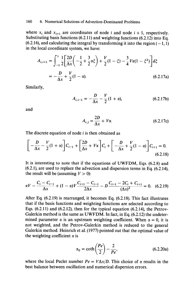
Ai.i+1 = f:1 ~[!~( -~ + ~~~) + ~(l-~) - ~ V~(1 - ~2)Jd~
D
V
= - Llx + 2(1 - ~).
(6.2.17a)
Similady,
D
V
A. . I = - - - - (1 + ~)
1,1Llx
2
'
(6.2. 17b)
and
2D
Ai,j = Llx + V~.
(6.2. 17c)
The discrete equation of node i is then obtained as
[ -:x -~(1 + ~)JCi-1 + [!~ + V~JCi + [ - :x + ~(1- ~)JCi+l = O.
(6.2.18)
It is interesting to note that if the equations of UWFDM, Eqs. (6.2.8) and
(6.2.1), are used to replace the advection and dispersion terms in Eq. (6.2.14),
the result will be (assuming V> 0):
V - Ci - Ci-I
(1 _ )V Ci +1 - Ci-I _ D Ci-I - 2Ci + Ci+1 = 0 '6219)
~
Llx
+
~
2Llx
(LlX)2
. ( ..
After Eq. (6.2.19) is rearranged, it becomes Eq. (6.2.18). This fact illustrates
that if the basis functions and weighting functions are selected according to
Eqs. (6.2.11) and (6.2.12), then for the typical equation (6.2.14), the PetrovGalerkin method is the same as UWFDM. In fact, in Eq. (6.2.12) the undetermined parameter ~ is an upstream weighting coefficient. When ~ = 0, it is
not weighted, and the Petrov-Galerkin method is reduced to the general
Galerkin method. Heinrich et al. (1977) pointed out that the optimal value of
the weighting coefficient ~ is
( pe) 2
~o = coth 2 - Pe'
(6.2.20a)
where the local Peclet number Pe = VLlx/D. This choice of ~ results in the
best balance between oscillation and numerical dispersion errors.
6. Numerical Solutions of Advection-Dominated Problems
where Xi and Xi+1 are coordinates of node i and node i + 1, respectively.
Substituting basis functions (6.2.11) and weighting functions (6.2.12) into Eq.
(6.2.16), and calculating the integral by transforming it into the region (-1,1)
in the local co ordinate system, we have:
Ai.i+1 = f:1 ~[!~( -~ + ~~~) + ~(l-~) - ~ V~(1 - ~2)Jd~
D
V
= - Llx + 2(1 - ~).
(6.2.17a)
Similady,
D
V
A. . I = - - - - (1 + ~)
1,1Llx
2
'
(6.2. 17b)
and
2D
Ai,j = Llx + V~.
(6.2. 17c)
The discrete equation of node i is then obtained as
[ -:x -~(1 + ~)JCi-1 + [!~ + V~JCi + [ - :x + ~(1- ~)JCi+l = O.
(6.2.18)
It is interesting to note that if the equations of UWFDM, Eqs. (6.2.8) and
(6.2.1), are used to replace the advection and dispersion terms in Eq. (6.2.14),
the result will be (assuming V> 0):
V - Ci - Ci-I
(1 _ )V Ci +1 - Ci-I _ D Ci-I - 2Ci + Ci+1 = 0 '6219)
~
Llx
+
~
2Llx
(LlX)2
. ( ..
After Eq. (6.2.19) is rearranged, it becomes Eq. (6.2.18). This fact illustrates
that if the basis functions and weighting functions are selected according to
Eqs. (6.2.11) and (6.2.12), then for the typical equation (6.2.14), the PetrovGalerkin method is the same as UWFDM. In fact, in Eq. (6.2.12) the undetermined parameter ~ is an upstream weighting coefficient. When ~ = 0, it is
not weighted, and the Petrov-Galerkin method is reduced to the general
Galerkin method. Heinrich et al. (1977) pointed out that the optimal value of
the weighting coefficient ~ is
( pe) 2
~o = coth 2 - Pe'
(6.2.20a)
where the local Peclet number Pe = VLlx/D. This choice of ~ results in the
best balance between oscillation and numerical dispersion errors.