

156
6. Numerical Solutions of Advection-Dominated Problems
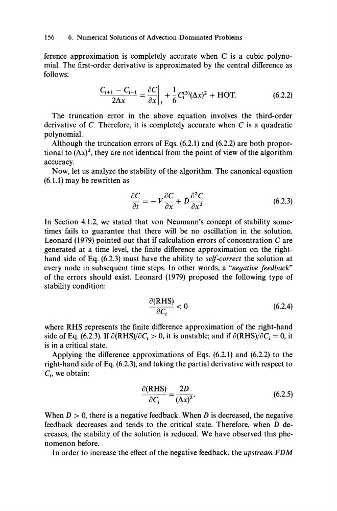
ference approximation is completely accurate when C is a cubic polynomial. The first-order derivative is approximated by the central difference as
folIows:
C i +1 - C i - 1 = OCI
~C!3)(L\)2 HOT
2L\x
OX . + 6 I X +
.
I
(6.2.2)
The truncation error in the above equation involves the third-order
derivative of C. Therefore, it is completely accurate when C is a quadratic
polynomial.
Although the truncation errors of Eqs. (6.2.1) and (6.2.2) are both proportional to (L\X)2, they are not identical from the point of view of the algorithm
accuracy.
Now, let us analyze the stability of the algorithm. The canonical equation
(6.1.1) may be rewritten as
(6.2.3)
In Section 4.1.2, we stated that von Neumann's concept of stability sometimes fails to guarantee that there will be no oscillation in the solution.
Leonard (1979) pointed out that if calculation errors of concentration C are
genera ted at a time level, the finite difference approximation on the righthand side of Eq. (6.2.3) must have the ability to self-correct the solution at
every node in subsequent time steps. In other words, a "negative feedback"
of the errors should exist. Leonard (1979) proposed the following type of
stability condition:
o(RHS) °
oe. <
I
(6.2.4)
where RHS represents the finite difference approximation of the right-hand
side of Eq. (6.2.3). If o(RHS)joC i > 0, it is unstable; and if o(RHS)joC i = 0, it
is in a critical state.
Applying the difference approximations of Eqs. (6.2.1) and (6.2.2) to the
right-hand side ofEq. (6.2.3), and taking the partial derivative with respect to
Ci' we obtain:
o(RHS)
2D
oC i = (L\X)2'
(6.2.5)
When D > 0, there is a negative feedback. When D is decreased, the negative
feedback decreases and tends to the critical state. Therefore, when D decreases, the stability of the solution is reduced. We have observed this phenomenon before.
In order to increase the effect of the negative feedback, the upstream F DM
6. Numerical Solutions of Advection-Dominated Problems
ference approximation is completely accurate when C is a cubic polynomial. The first-order derivative is approximated by the central difference as
folIows:
C i +1 - C i - 1 = OCI
~C!3)(L\)2 HOT
2L\x
OX . + 6 I X +
.
I
(6.2.2)
The truncation error in the above equation involves the third-order
derivative of C. Therefore, it is completely accurate when C is a quadratic
polynomial.
Although the truncation errors of Eqs. (6.2.1) and (6.2.2) are both proportional to (L\X)2, they are not identical from the point of view of the algorithm
accuracy.
Now, let us analyze the stability of the algorithm. The canonical equation
(6.1.1) may be rewritten as
(6.2.3)
In Section 4.1.2, we stated that von Neumann's concept of stability sometimes fails to guarantee that there will be no oscillation in the solution.
Leonard (1979) pointed out that if calculation errors of concentration C are
genera ted at a time level, the finite difference approximation on the righthand side of Eq. (6.2.3) must have the ability to self-correct the solution at
every node in subsequent time steps. In other words, a "negative feedback"
of the errors should exist. Leonard (1979) proposed the following type of
stability condition:
o(RHS) °
oe. <
I
(6.2.4)
where RHS represents the finite difference approximation of the right-hand
side of Eq. (6.2.3). If o(RHS)joC i > 0, it is unstable; and if o(RHS)joC i = 0, it
is in a critical state.
Applying the difference approximations of Eqs. (6.2.1) and (6.2.2) to the
right-hand side ofEq. (6.2.3), and taking the partial derivative with respect to
Ci' we obtain:
o(RHS)
2D
oC i = (L\X)2'
(6.2.5)
When D > 0, there is a negative feedback. When D is decreased, the negative
feedback decreases and tends to the critical state. Therefore, when D decreases, the stability of the solution is reduced. We have observed this phenomenon before.
In order to increase the effect of the negative feedback, the upstream F DM