

5.4. The Solution of Finite Element Systems
143
When Eq. (5.3.45) is listed for all nodes where the concentration is unknown, a system of discrete equations are obtained.
The advantages of the three-dimensional MCBM are that the coefficients
of the discrete equations are given explicitly, and we do not need to assume
that direction z is a principal direction of dispersion.
Some numerical examples of three-dimensional MCBM can be found in
Wang et al. (1986).
5.4 The Solution of Finite Element Systems
5.4.1 Features of Finite Element Systems and
Direct Solutions
We have seen that, no matter what kind of FEM is used in the discretization
of space variables, the advection-dispersion equation will be tranferred into a
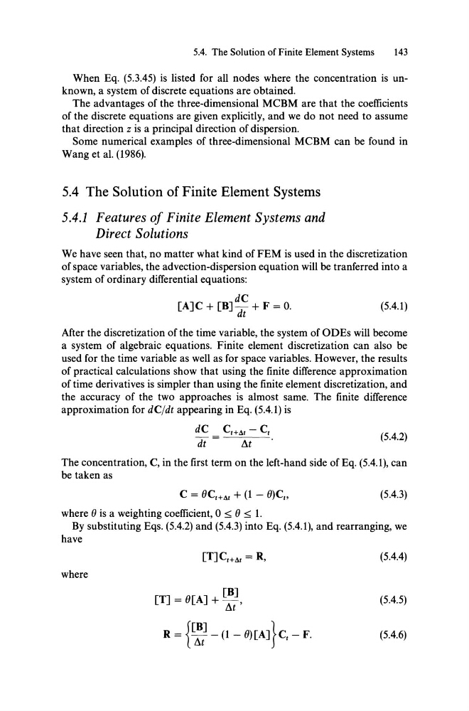
system of ordinary differential equations:
dC
[A]C + [B]Tt + F = O.
(5.4.1)
After the discretization of the time variable, the system of ODEs will become
a system of algebraic equations. Finite element discretization can also be
used for the time variable as weIl as for space variables. However, the results
of practical calculations show that using the finite difference approximation
of time derivatives is simpler than using the finite element discretization, and
the accuracy of the two approaches is almost same. The finite difference
approximation for dCjdt appearing in Eq. (5.4.1) is
dC Ct+41 - CI
Tt= M
(5.4.2)
The concentration, C, in the first term on the left-hand side of Eq. (5.4.1), can
be taken as
C = OCtHt + (1 - O)Ct ,
(5.4.3)
where 0 is a weighting coefficient, 0 :s;; 0 :s;; 1.
By substituting Eqs. (5.4.2) and (5.4.3) into Eq. (5.4.1), and rearranging, we
have
[T]C tHt = R,
(5.4.4)
where
[T] = O[A] + [::'
(5.4.5)
{ [B]
}
R= Tt-(1-0)[A] Ct-F.
(5.4.6)
143
When Eq. (5.3.45) is listed for all nodes where the concentration is unknown, a system of discrete equations are obtained.
The advantages of the three-dimensional MCBM are that the coefficients
of the discrete equations are given explicitly, and we do not need to assume
that direction z is a principal direction of dispersion.
Some numerical examples of three-dimensional MCBM can be found in
Wang et al. (1986).
5.4 The Solution of Finite Element Systems
5.4.1 Features of Finite Element Systems and
Direct Solutions
We have seen that, no matter what kind of FEM is used in the discretization
of space variables, the advection-dispersion equation will be tranferred into a
system of ordinary differential equations:
dC
[A]C + [B]Tt + F = O.
(5.4.1)
After the discretization of the time variable, the system of ODEs will become
a system of algebraic equations. Finite element discretization can also be
used for the time variable as weIl as for space variables. However, the results
of practical calculations show that using the finite difference approximation
of time derivatives is simpler than using the finite element discretization, and
the accuracy of the two approaches is almost same. The finite difference
approximation for dCjdt appearing in Eq. (5.4.1) is
dC Ct+41 - CI
Tt= M
(5.4.2)
The concentration, C, in the first term on the left-hand side of Eq. (5.4.1), can
be taken as
C = OCtHt + (1 - O)Ct ,
(5.4.3)
where 0 is a weighting coefficient, 0 :s;; 0 :s;; 1.
By substituting Eqs. (5.4.2) and (5.4.3) into Eq. (5.4.1), and rearranging, we
have
[T]C tHt = R,
(5.4.4)
where
[T] = O[A] + [::'
(5.4.5)
{ [B]
}
R= Tt-(1-0)[A] Ct-F.
(5.4.6)